The world of DevOps and container orchestration is constantly changing, and picking the right tool can make a big difference in how efficiently microservices are deployed. One tool that stands out is HashiCorp Nomad. In this guide, we’ll dive into how you can deploy a simple microservice using Nomad on a DigitalOcean Droplet running Ubuntu server.
Nomad is a lightweight workload scheduler that manages application deployment and scaling across a cluster of machines. It supports multiple workload types, integrates with other HashiCorp tools, and is infrastructure agnostic. Nomad’s simplicity, versatility, scalability, resource efficiency, and integration make it an excellent choice for deploying and managing microservices.
Check out Nomad’s official documentation and its Comparison guide for more details and features.
Before we begin, make sure you have the following installed:
Or
First and foremost, you will need to get the SSH-key-id and Access Token, which will be used to run the doctl
command to create a Droplet.
Let’s set things up:
doctl compute ssh-key list
Now, let’s create an Ubuntu Droplet:
doctl compute droplet create my-droplet --size s-2vcpu-4gb --region nyc1 --image ubuntu-22-04-x64 --ssh-keys <YOUR_SSH_KEY_ID> --access-token '<ACCESS_TOKEN>' --output json"
The above command creates a new DigitalOcean Droplet named “my-droplet” with a specified size, region, image,SSH key ID and access token.
You can use the following command to get the supported sizes for Droplets and their hourly and monthly prices:
doctl compute size list
You can refer to the doctl
commands reference to learn more and play around with doctl
.
Now, to SSH into your Ubuntu Droplet, we will first need the Public IP of the Droplet, which can be found using the following doctl
command:
doctl compute droplet get my-droplet
Note the Public IPv4 address from the above command and then SSH to the Droplet from your local server.
Once you know the Public IPv4 address of your Ubuntu Droplet, you will need to add SSH keys to connect to your Droplet remotely from your local system via SSH.
Now that you have added your SSH keys, you can log in to the Ubuntu Droplet remotely via SSH:
ssh root@<PUBLIC_IP>
You can refer to the following guides to install Nomad and Docker engine on an Ubuntu server:
Nomad installed on your DigitalOcean Ubuntu Droplet.
Docker Engine installed and running on your Ubuntu Droplet.
Once you have the Ubuntu Droplet deployed with Nomad and Docker installed, you can start Nomad in “dev mode” using the following command in the terminal:
nomad agent -dev
You will observe an output like the one below:
Output==> No configuration files loaded
==> Starting Nomad agent...
==> Nomad agent configuration:
Advertise Addrs: HTTP: 127.0.0.1:4646; RPC: 127.0.0.1:4647; Serf: 127.0.0.1:4648
Bind Addrs: HTTP: [127.0.0.1:4646]; RPC: 127.0.0.1:4647; Serf: 127.0.0.1:4648
Client: true
Log Level: DEBUG
Node Id: 51b0f49b-564b-5d1c-8e99-a17336c2a597
Region: Global (DC: dc1)
Server: true
Version: 1.6.2
==> Nomad agent started! Log data will stream in below:
2023-12-05T18:43:58.414+0530 [INFO] nomad.raft: initial configuration: index=1 servers="[{Suffrage:Voter ID:e707dbd2-be06-7cfc-dff0-a11714eec76f Address:127.0.0.1:4647}]"
2023-12-05T18:43:58.415+0530 [INFO] nomad.raft: entering follower state: follower="Node at 127.0.0.1:4647 [Follower]" leader-address= leader-id=
This will start the Nomad agent on your machine as the server and client components. In dev mode, Nomad runs on a single node and does not persist in any data, making it ideal for experimentation and development.
Once the Nomad agent starts running, you can access the Nomad web user interface by visiting http://localhost:4646 in your browser. In our case, we need some tunneling to access the Nomad UI from our Ubuntu Server. We can use Pinggy, a tool that provides Public URLs for Localhost. It generates a temporary URL through which one can access the Nomad UI.
ssh -p 443 -R0:localhost:4646 -L4300:localhost:4300 qr@a.pinggy.io
Copy and run the above SSH command on your Ubuntu server to get Nomad UI URLs that can be accessed from your phone browser or any other device.
Copy the URLs displayed in the above screenshot.
Here is the Nomad UI. You can view the Job details, details of the deployment, etc, from this UI throughout the tutorial.
Nomad jobs are defined by the Nomad job specification, also known as “jobspec”. The job spec schema is written in HCL.
The job specification is divided into smaller sections, which you can find in the navigation menu. Nomad HCL is parsed in the command line and then sent to Nomad in JSON format via the HTTP API.
Let’s talk about each in a bit more detail:
task - Nomad uses tasks as the smallest unit of work. These tasks are executed by task drivers such as docker or exec, which allow Nomad to be flexible in the tasks it supports. Tasks specify their required task driver, configuration for the driver, constraints, and resources required.
group -A group refers to a set of tasks that are executed on a single Nomad client."
Job - A job is the core unit of control for Nomad and defines the application and its configurations. It can contain one or many tasks.
job specification - A job specification, also known as a jobspec defines the schema for Nomad jobs. This describes the type of job, the tasks and resources necessary for the job to run, job information like which clients it can run on, and more.
allocation - An allocation is a mapping between a task group in a job and a client node. When a job is run, Nomad will choose a client capable of running it and allocate resources on the machine for the task(s) in the task group defined in the job.
The above constructs make up a Job in Nomad.
Now that Nomad is operational, we can schedule our first job. Our initial task will involve running the http-echo
Docker container. This straightforward application generates an HTML page displaying the arguments passed to the http-echo process, such as “Hello World”. The process dynamically listens on a port specified by another argument.
Let’s create a job file that ends with the name “microservice.nomad”—all the job files in Nomad end with .nomad
suffix .
job "http-microservice" {
datacenters = ["dc1"]
group "echo" {
count = 1
task "server" {
driver = "docker"
config {
image = "hashicorp/http-echo:latest"
args = [
"-listen", ":${NOMAD_PORT_http}",
"-text", "Hello and welcome to ${NOMAD_IP_http} running on port ${NOMAD_PORT_http}. This is my first microservice deployment using Nomad.",
]
}
resources {
network {
mbits = 10
port "http" {}
}
}
}
}
}
In this example, we defined a job called http-microservice
, set the driver to use docker
, and passed the necessary text and port arguments to the container. As we need network access to the container to display the resulting webpage, we define the resources section as requiring a network with a port that Nomad dynamically chooses from the host machine to the container during runtime.
Nomad supports using dynamic port assignment, i.e., you don’t need to specify a port.
We can submit/run
new or update existing jobs with the nomad job run
command, using job files that conform to the job specification format.
nomad job run microservice.nomad
Output:
Output==> 2023-12-06T13:58:25+05:30: Monitoring evaluation "bd6dd191"
2023-12-06T13:58:25+05:30: Evaluation triggered by job "http-microservice"
2023-12-06T13:58:25+05:30: Evaluation within deployment: "b8499a02"
2023-12-06T13:58:25+05:30: Evaluation status changed: "pending" -> "complete"
==> 2023-12-06T13:58:25+05:30: Evaluation "bd6dd191" finished with status "complete"
==> 2023-12-06T13:58:25+05:30: Monitoring deployment "b8499a02"
✓ Deployment "b8499a02" successful
2023-12-06T13:58:25+05:30
ID = b8499a02
Job ID = http-microservice
Job Version = 0
Status = successful
Description = Deployment completed successfully
Deployed
Task Group Desired Placed Healthy Unhealthy Progress
Deadline
echo 1 1 1 0
2023-12-06T14:08:23+05:30
We can check the status of a job using the command:
nomad job status http-microservice
OutputID = http-microservice
Name = http-microservice
Submit Date = 2023-12-13T13:44:55+05:30
Type = service
Priority = 50
Datacenters = dc1
Namespace = default
Node Pool = default
Status = running
Periodic = false
Parameterized = false
Summary
Task Group Queued Starting Running Failed Complete Lost Unknown
echo 0 0 1 0 0 0 0
Latest Deployment
ID = 9a72c817
Status = successful
Description = Deployment completed successfully
Deployed
Task Group Desired Placed Healthy Unhealthy Progress Deadline
echo 1 1 1 0 2023-12-13T14:00:33+05:30
Allocations
ID Node ID Task Group Version Desired Status Created Modified
84d70c8f aa3f6a1a echo 0 run running 5m19s ago 5m6s ago
Please make a note of the allocation ID in the above output:84d70c8f. Allocation ID is used to troubleshoot deployment issues in Nomad.
You can also access the Nomad UI using the below command to check the Jobs and other important details of your deployment on your local desktop:
nomad ui <job_name>
In our case:
nomad ui http-microservice
We can use the command nomad alloc-status <allocation_id>
to get the port on which the microservice is deployed. When deploying jobs with dynamic ports, finding the exact port on which a specific task has been deployed can be challenging because the port is dynamically allocated at runtime. This command is also great for troubleshooting any deployment issues in Nomad.
We can get the allocation_id using the command nomad job status http-microservice
specified in the above section.
nomad alloc-status 84d70c8f
Output:
OutputID = 84d70c8f-0687-e1c7-27fe-172ae274580b
Eval ID = 404f0d71
Name = http-microservice.echo[0]
Node ID = aa3f6a1a
Node Name = XXXXXXXX
Job ID = http-microservice
Job Version = 0
Client Status = running
Client Description = Tasks are running
Desired Status = run
Desired Description = <none>
Created = 11m3s ago
Modified = 10m50s ago
Deployment ID = 9a72c817
Deployment Health = healthy
Task "server" is "running"
Task Resources:
CPU Memory Disk Addresses
0/100 MHz 9.0 MiB/300 MiB 300 MiB http: 127.0.0.1:20004
Task Events:
Started At = 2023-12-13T08:20:23Z
Finished At = N/A
Total Restarts = 0
Last Restart = N/A
Recent Events:
Time Type Description
2023-12-13T13:50:23+05:30 Started Task started by client
2023-12-13T13:50:20+05:30 Driver Downloading image
2023-12-13T13:50:19+05:30 Task Setup Building Task Directory
2023-12-13T13:50:19+05:30 Received Task received by client
From the above, we can make a note of the address on which the microservice is running, which is 127.0.0.1:20004
, and send a curl request to get the status of the microservice.
curl -i 127.0.0.1:20004
Outputcurl: (56) Recv failure: Connection reset by peer
anish@W2MK93VGYX nomad.d % curl -i http://127.0.0.1:20004
HTTP/1.1 200 OK
X-App-Name: http-echo
X-App-Version: 1.0.0
Date: Wed, 13 Dec 2023 08:24:59 GMT
Content-Length: 108
Content-Type: text/plain; charset=utf-8
Hello and welcome to 127.0.0.1 running on port 20004. This is my first microservice deployment using Nomad.
We can verify that the microservice has been successfully deployed from the above.
One of the key benefits of using Nomad is its ability to scale your microservices based on demand. To scale up your job, simply modify the job file to increase the count
parameter or use the nomad job scale <job> <count>
command.
Let’s scale our hello-world microservice:
nomad job scale http-microservice 3
Output:
Output 2023-12-05T19:28:45+05:30: Evaluation status changed: "pending" -> "complete
==> 2023-12-05T19:28:45+05:30: Evaluation "84241aca" finished with status "complete"
==> 2023-12-05T19:28:45+05:30: Monitoring deployment "a26236c7"
✓ Deployment "a26236c7" successful
2023-12-05T19:28:58+05:30
ID = a26236c7
Job ID = http-microservice
Job Version = 1
Status = successful
Description = Deployment completed successfully
Deployed
Task Group Desired Placed Healthy Unhealthy Progress
Deadline
echo 3 3 3 0
2023-12-05T19:38:57+05:30**
On the Nomad UI(http://localhost:4646/ui/jobs
), we can see the changes being reflected on the go:
Nomad offers a range of advanced features and concepts that can further enhance your deployment strategy:
1. Task Drivers:
Nomad supports multiple task drivers, allowing you to choose the best runtime environment for your applications. Explore different task drivers for various workload types.
2. Task Groups:
Organize your tasks into groups for logical separation and resource allocation. Task groups enable you to define specific constraints and settings for different sets of tasks.
3. Update Policies:
Nomad provides flexible update policies for controlling how your jobs are updated. Explore strategies like rolling updates to ensure zero downtime during deployments.
4. Service Discovery:
Utilize Nomad’s integration with Consul for seamless service discovery. This is crucial for dynamic microservices architectures where services need to locate and communicate with each other.
Congratulations! You’ve successfully deployed a simple microservice and explored some advanced features of Nomad. Nomad’s simplicity, versatility, and integration capabilities make it a compelling choice for DevOps engineers managing microservices at scale. Consider exploring more features and integrating Nomad into your broader infrastructure to maximize efficiency and scalability.
You can check out Nomad’s tutorial library and its comprehensive and detailed introduction guide to gain deeper insights into using Nomad.
]]>I have copied:
When I use the command to start the service from droplet ssh session and I check the status, the system shows this information:
● webserver-0.0.1-SNAPSHOT.service - Webserver 03motorsport Spring Boot Application
Loaded: loaded (/etc/systemd/system/webserver-0.0.1-SNAPSHOT.service; enabled; vendor preset: enabled)
Active: activating (auto-restart) (Result: exit-code) since Fri 2023-10-27 16:40:29 UTC; 396ms ago
Process: 13162 ExecStart=/usr/bin/java -jar /artifact/webserver-0.0.1-SNAPSHOT.jar (code=exited, status=1/FAILURE)
Main PID: 13162 (code=exited, status=1/FAILURE)
CPU: 1ms
The service remains in “activating” status, and my web server is not loading properly.
What I am doing wrong?
Thanks in advance for the help :)
Gianluca
]]>Let me explain you in detail. I have a form in which I entered some parameter for my bot and when I click on start bot the bot will start with those entered parameter and redirect back to form page after starting bot. I need to run 2000-2500 bots in background even user shutdown their PC/Laptop.
Which tech stack I have to use to achieve these goals?
]]>[myfrontend-app] [2023-01-23 17:55:44] 2023/01/23 17:55:44 [error] 20#20: *9 SSL_do_handshake() failed (SSL: error:1408F10B:SSL routines:ssl3_get_record:wrong version number) while SSL handshaking to upstream, client: 10.33.44.55, server: , request: "POST /api/v1/auth/tokens/ HTTP/1.1", upstream: "https://104.11.211.77:80/api/v1/auth/tokens/", host: "myfrontend-app-abcdef.ondigitalocean.app", referrer: "https://myfrontend-app-abcdef.ondigitalocean.app/login"
Here is my nginx conf
upstream be-app-1 {
server be-app-1-abc.ondigitalocean.app;
}
upstream be-app-2 {
server be-app-2-def.ondigitalocean.app;
}
upstream be-app-3 {
server be-app-3-ghi.ondigitalocean.app;
}
server {
listen 80;
listen [::]:80;
# The root directory of the Vue.js application
root /usr/share/nginx/html;
# Serve the index.html file for all requests
index index.html;
# Serve the Vue.js application's static files
location / {
try_files $uri $uri/ /index.html;
}
location ~ ^/api/v1/auth/(.*) {
proxy_pass https://be-app-1/api/v1/auth/$1;
proxy_set_header Host $host;
proxy_set_header X-Real-IP $remote_addr;
proxy_set_header X-Forwarded-For $proxy_add_x_forwarded_for;
proxy_set_header X-Forwarded-Proto https;
proxy_ssl_server_name on;
}
location ~ ^/api/v1/pro/(.*) {
# using $1 in the target. Example; offenders/ AND $is_args$arg are for Http query params
proxy_pass https://be-app-2/api/v1/pro/$1$is_args$args;
proxy_set_header Host $host;
proxy_set_header X-Real-IP $remote_addr;
proxy_set_header X-Forwarded-For $proxy_add_x_forwarded_for;
proxy_set_header X-Forwarded-Proto https;
}
location ~ ^/api/v1/vro/(.*) {
proxy_pass https://be-app-3/api/v1/vro/$1$is_args$args;
proxy_set_header Host $host;
proxy_set_header X-Real-IP $remote_addr;
proxy_set_header X-Forwarded-For $proxy_add_x_forwarded_for;
proxy_set_header X-Forwarded-Proto https;
}
}
Any help would be great!
]]>Instead of returning file from microservice (they can be big and our transport protocol handle only 1mb messages) we are storing file locally and just simply return link to our API which downloads it.
Now we have problem with app platform because we can’t get this file from another service.
We would not like to use spaces, because it takes precious miliseconds for uploading the file.
Is there a way we can access filed on microservice from our API?
Thanks!
]]>Recently I’ve started using digital ocean app platform for setting microservice based architecture for my startup but I’m having issues with horizontal scalling.
At the time I have:
They are communicating through TCP, but the problem is that only one instance of microservice is used to do the hard work, the second one never gets any traffic.
What can I do with this situation?
]]>On my local environment everything works perfectly, but when I try to set up same architecture on digitalocean apps I get Error: connect ECONNREFUSED
My app spec looks like this:
services:
- build_command: npm run build
environment_slug: node-js
gitlab:
branch: develop
deploy_on_push: true
repo: html-pdf/html-pdf-api
http_port: 8080
instance_count: 1
instance_size_slug: basic-xxs
name: dev-html-pdf-api
routes:
- path: /
run_command: npm run start:prod
source_dir: /
- dockerfile_path: Dockerfile
gitlab:
branch: develop
deploy_on_push: true
repo: html-pdf/html-pdf-microservice
http_port: 8080
instance_count: 1
instance_size_slug: basic-xxs
internal_ports:
- 3000
name: dev-html-pdf-microservice
routes:
- path: /microservice
run_command: npm run start:prod
source_dir: /
so as you can see I’ve enabled 3000 internal port.
About the code, microservice is set up to listen on localhost:3000, and the main api is connecting to it using options:
options: {
host: 'dev-html-pdf-microservice',
port: 3000,
}
Unfortunately I get Error: connect ECONNREFUSED 10.245.138.142:3000. I’ve tried many other options with different options on api and microservice but same result.
]]>Serverless architecture allows backend web services to be implemented on an as-needed basis. Rather than having to maintain your own server configuration, architecting your software for serverless providers can minimize the overhead involved. Serverless applications are typically deployed from a Git repository into an environment that can scale up or down as needed.
Serverless deployments usually involve microservices. Using microservices is an approach to software architecture that structures an application as a collection of services that are loosely coupled, independently deployable, and independently maintainable and testable. Microservice architectures predate the widespread use of serverless deployments, but they are a natural fit together. Microservices can be used in any context that allows them to be deployed independently and managed by a central process or job server. Serverless implementations abstract away this central process management, leaving you to focus on your application logic.
This tutorial will review some best practices for rearchitecting monolithic applications to use microservices.
Rearchitecting, or refactoring, a monolithic application, is often invisible by design. If you plan to significantly rewrite your application logic while introducing no new features, your goal should be to avoid service disruptions to the greatest extent possible. This can entail using some form of blue-green deployment. When implementing microservices, it usually also entails replacing your application’s functionality on a step-by-step basis. This requires you to thoroughly implement unit tests to ensure that your application gracefully handles any unexpected edge cases. It also provides many opportunities to review your application logic and evaluate how to replace existing features with distinct microservices.
Microservices are equally well-supported by almost all major programming languages, and adopting a microservice-driven architecture can facilitate combining multiple different languages or frameworks within the same project. This allows you to adopt the best possible solution for each component of your stack, but can also change the way that you think about code maintenance.
Some architectures are a more natural fit for microservices than others. If your application logic contains multiple sequential steps that all depend on one another, it may not be a good idea to abstract each of them into individual microservices. In that case, you would need a sophisticated controller architecture that could handle and route any mid-stage errors. This is possible with a microservice architecture that uses a framework like Gearman to dispatch subprocesses, but it is more inconvenient when working with serverless deployments and can add complexity without necessarily solving problems.
Instead of delineating microservices between stages of the same input processing pipeline, you could delineate microservices between application state changes, or every time some output is returned to a user. This way, you do not need to pass the same data between public API calls as part of a single process. Handling your application state can be challenging with a microservice architecture, because each microservice will only have access to its own input, rather than to a globally defined scope. Wherever possible, you should create and pass similar data structures to each of your microservices, so that you can make reliable assumptions about the scope available to each of them.
Consider creating and maintaining your own application libraries for core logic and functions that are likely to be used in multiple places, and then create microservices which join together unique combinations of this logic. Remember that microservices can scale to zero: there is no penalty from maintaining unused code paths. This way, you can create microservices which do not directly depend on other microservices, because they each include a complete, linear set of application logic, composed of function calls which you maintain in a separate repository.
When working with microservices, you should employ the principles of GitOps as much as possible. Treat Git repositories as a single source of truth for deployment purposes. Most language-specific package managers, such as pip
for Python and npm
for Node.js, provide syntax to deploy packages from your own Git repositories. This can be used in addition to the default functionality of installing from PyPI
, npmjs.com
or other upstream repositories. This way, you can gracefully combine your own in-development functions with third-party libraries without deviating from best practices around maintainability or reproducibility.
Each of your microservices can implement its own API, and depending on the complexity of your application, you can implement another API layer on top of that (and so on, and so on), and plan to only expose the highest-level API to your users. Although maintaining multiple different API routes can add complexity, this complexity can be resolved through good documentation of each of your individual microservices’ API endpoints. Communicating between processes using well-defined API calls, such as HTTP GET
and POST
, adds virtually no overhead and will make your microservices much more reusable than if they used more idiosyncratic interprocess communication.
Adopting microservices may naturally push you toward also adopting more Software-as-a-Service (SaaS) tooling as a drop-in replacement for various parts of your application stack. This is almost always good in principle. While you are under no obligation to replace your own function calls with third-party services, retaining the option to do so will keep your application logic more flexible and more contemporary.
Effectively migrating to Microservices requires you to synthesize a number of best practices around software development and deployment.
When rearchitecting an application to use microservices, you should follow the best practices for Continuous Integration and Continuous Delivery to incrementally replace features of your monolithic architecture. For example, you can use branching by abstraction — building an abstraction layer within an existing implementation so that a new implementation can be built out behind the abstraction in parallel — to refactor production code without any disruption to users. You can also use decorators, a language feature of TypeScript and Python, to add more code paths to existing functions. This way, you can progressively toggle or roll back functionality.
Microservices have become popular at the same time as containerization frameworks like Docker for good reason. They have similar goals and architectural assumptions:
Containers provide process and dependency isolation so that they can be deployed on an individual basis.
Containers allow other applications running in tandem with them to function as a “black box” — they don’t need to share state or any information other than input and output.
Container registries, such as Docker Hub, make it possible to publish and use your own dependencies interchangeably with third-party dependencies.
In theory, your microservices should be equally suited to running in a Docker container or a Kubernetes cluster as they are in a serverless deployment. In practice, there may be significant advantages to one or the other. Highly CPU-intensive microservices such as video processing may not be economical in serverless environments, whereas maintaining a Kubernetes control plane and configuration details requires a significant commitment. However, building with portability in mind is always a worthwhile investment. Depending on the complexity of your architecture, you may be able to support multiple environments merely by creating the relevant .yml
metadata declarations and Dockerfile
s. Prototyping for both Kubernetes and serverless environments can improve the overall resilience of your architecture.
Generally speaking, you should not need to worry about database concurrency or other storage scaling issues inside of microservices themselves. Any relevant optimizations should be addressed and implemented directly by your database, your database abstraction layer, or your Database-as-a-Service (DBaaS) provider, so that your microservices can perform any create-read-update-delete (CRUD) operations without embellishment. Microservices must be able to concurrently query and update the same data sources, and your database backend should support these assumptions.
When making breaking, non-backwards-compatible updates to your microservices, you should provide new endpoints. For example, you might provide a /my/service/v2
in addition to a preexisting /my/service/v1
, and plan to gradually deprecate the /v1
endpoint. This is important because production microservices are likely to become useful and supported outside of their originally intended context. For this reason, many serverless providers will automatically version your URL endpoints to /v1
when deploying new functions.
Implementing microservices in your application can replace nested function calls or private methods by promoting them to their own standalone service. Take this example of a Flask application, which performs a Google query based on a user’s input into a web form, then manipulates the result before returning it back to the user:
from flask import *
from flask import render_template
from flask import Markup
from googleapiclient.discovery import build
from config import *
app = Flask(__name__)
def google_query(query, api_key, cse_id, **kwargs):
query_service = build("customsearch", "v1", developerKey=api_key)
query_results = query_service.cse().list(q=query, cx=cse_id, **kwargs).execute()
return query_results['items']
def manipulate_result(input, cli=False):
search_results = google_query(input, keys["api_key"], keys["cse_id"])
for result in search_results:
abc(result)
…
return manipulated_text
@app.route('/<string:text>', methods= ["GET"])
def get_url(text):
manipulated_text = manipulate_result(text)
return render_template('index.html', prefill=text, value=Markup(manipulated_text))
if __name__ == "__main__":
serve(app, host='0.0.0.0', port=5000)
This application provides its own web endpoint, which includes an HTTP GET
method. Providing a text string to that endpoint calls a function called manipulate_result()
, which first sends the text to another function google_query()
, then manipulates the text from the query results before returning it to the user.
This application could be refactored into two separate microservices, both of which take HTTP GET
parameters as input arguments. The first would return Google query results based on some input, using the googleapiclient
Python library:
from googleapiclient.discovery import build
from config import *
def main(input_text):
query_service = build("customsearch", "v1", developerKey=api_key)
query_results = query_service.cse().list(q=query, cx=cse_id, **kwargs).execute()
return query_results['items']
A second microservice would then manipulate and extract the relevant data to be returned to the user from those search results:
import requests
def main(search_string, standalone=True):
if standalone == False:
search_results = requests.get('https://path/to/microservice_1/v1/'+search_string).text
else:
search_results = search_string
for result in search_results:
abc(result)
…
return manipulated_text
In this example, microservice_2.py
performs all of the input handling, and calls microservice_1.py
directly via an HTTP post if an additional argument, standalone=False
has been provided. You could optionally create a separate, third function to join both microservices together, if you preferred to keep them entirely separate, but still provide their full functionality with a single API call.
This is a straightforward example, and the original Flask code does not appear to present a significant maintenance burden, but there are still advantages to being able to remove Flask from your stack. If you no longer need to run your own web request handler, you could then return these results to a static site, using a Jamstack environment, rather than needing to maintain a Flask backend.
In this tutorial, you reviewed some best practices for migrating monolithic applications to microservices, and followed a brief example for decomposing a Flask application into two separate microservice endpoints.
Next, you may want to learn more about efficient monitoring of microservice architectures to better understand the optimization of serverless deployments. You may also want to understand how to write a serverless function.
]]>Serverless architecture allows backend web services to be implemented on an as-needed basis. Rather than needing to maintain your own server configuration, architecting your software for serverless providers can minimize the overhead involved. Serverless applications are typically deployed from a Git repository into an environment that can scale up or down as needed.
This means that serverless functions can effectively “scale to zero” – a function or endpoint should consume no resources at all as long as it is not being accessed. However, this also means that serverless functions must be well-behaved, and should become available from an idle state only to provide individual responses to input requests. These responses can be as computationally intensive as needed, but must be invoked and terminated in a predictable manner.
This tutorial will cover some best practices for writing an example serverless function.
To follow this tutorial, you will need:
A local shell environment with a serverless deployment tool installed. Some serverless platforms make use of the serverless
command, while this tutorial will reflect DigitalOcean’s doctl sandbox
tools. Both provide similar functionality. To install and configure doctl
, refer to its documentation.
The version control tool Git available in your development environment. If you are working in Ubuntu, you can refer to installing Git on Ubuntu 20.04
A complete serverless application can be contained in only two files at a minimum — the configuration file, usually using .yml
syntax, which declares necessary metadata for your application to the serverless provider, and a file containing the code itself, e.g. my_app.py
, my_app.js
, or my_app.go
. If your application has any language dependencies, it will typically also declare them using standard language conventions, such as a package.json
file for Node.js.
To initialize a serverless application, you can use doctl sandbox init
with the name of a new directory:
- doctl sandbox init myServerlessProject
OutputA local sandbox area 'myServerlessProject' was created for you.
You may deploy it by running the command shown on the next line:
doctl sandbox deploy myServerlessProject
By default, this will create a project with the following directory structure:
myServerlessProject/
├── packages
│ └── sample
│ └── hello
│ └── hello.js
└── project.yml
project.yml
is contained in the top-level directory. It declares metadata for hello.js
, which contains a single function. All serverless applications will follow this same essential structure. You can find more examples, using other serverless frameworks, at the official Serverless Framework GitHub repository, or refer to DigitalOcean’s documentation. You can also create these directory structures from scratch without relying on an init
function, but note that the requirements of each serverless provider will differ slightly.
In the next step, you’ll explore the sample project you initialized in greater detail.
A serverless application can be a single function, written in a language that is interpreted by your serverless computing provider (usually Go, Python, and JavaScript), as long as it can return
some output. Your function can call other functions or load other language libraries, but there should always be a single main function defined in your project configuration file that communicates with the endpoint itself.
Running doctl sandbox init
in the last step automatically generated a sample project for your serverless application, including a file called hello.js
. You can open that file using nano
or your favorite text editor:
- nano myServerlessProject/packages/sample/hello/hello.js
function main(args) {
let name = args.name || 'stranger'
let greeting = 'Hello ' + name + '!'
console.log(greeting)
return {"body": greeting}
}
This file contains a single function, called main()
, which can accept a set of arguments. This is the default way that serverless architectures manage input handling. Serverless functions do not necessarily need to directly parse JSON or HTTP headers to handle input. On most providers’ platforms, serverless functions will receive input from HTTP requests as a list of arguments that can be unpacked using standard language features.
The first line of the function uses JavaScript’s ||
OR operator to parse a name
argument if it is present, or use the string stranger
if the function is called without any arguments. This is important in the event that your function’s endpoint is queried incorrectly, or with missing data. Serverless functions should always have a code path that allows you to quickly return null
, or return the equivalent of null
in a well-formed HTTP response, with a minimum of additional processing. The next line, let greeting =
, performs some additional string manipulation.
Depending on your serverless provider, you may not have any filesystem or OS-level features available to your function. Serverless applications are not necessarily stateless. However, features that allow serverless applications to record or retain their state between runs are typically proprietary to each provider. The most common exception to this is the ability to log output from your functions. The sample hello.js
app contains a console.log()
function, which uses a built-in feature of JavaScript to output some additional data to a browser console or a local terminal’s stdout
without returning it to the user. Most serverless providers will allow you to retain and review logging output in this way.
The final line of the function is used to return
output from your function. Because most serverless functions are deployed as HTTP endpoints, you will usually want to return an HTTP response. Your serverless environment may automatically scaffold this response for you. In this case, it is only necessary to return a request body
within an array, and the endpoint configuration takes care of the rest.
This function could perform many more steps, as long as it maintained the same baseline expectations around input and output. Alternatively, your application could run multiple serverless functions in a sequence, and they could be swapped out as needed. Serverless functions can be thought of as being similar to microservice-driven architectures: both enable you to construct an application out of multiple loosely-coupled services which are not necessarily dependent on one another, and communicate over established protocols such as HTTP. Not all microservice architectures are serverless, but most serverless architectures implement microservices.
Now that you understand the application architecture, in the next step, you’ll learn some best practices around preparing serverless functions for deployment and deploying serverless functions.
The doctl sandbox
command line tools allow you to deploy and test your application without promoting them to production, and other serverless implementations provide similar functionality. However, nearly all serverless deployment workflows will eventually involve you committing your application to a source control repository such as GitHub, and connecting the GitHub repository to your serverless provider.
When you are ready for a production deployment, you should be able to visit your serverless provider’s console and identify your source repository as a component of an application. Your application may also have other components, such as a static site, or it may just provide the one endpoint.
For now, you can deploy directly to a testing sandbox using doctl sandbox
:
- doctl sandbox deploy myServerlessProject
This will return information about your deployment, including another command that you can run to request your live testing URL:
OutputDeployed '~/Desktop/myServerlessProject'
to namespace 'f8572f2a-swev6f2t3bs'
on host 'https://faas-nyc1-78edc.doserverless.io'
Deployment status recorded in 'myServerlessProject\.nimbella'
Deployed functions ('doctl sbx fn get <funcName> --url' for URL):
- sample/hello
Running this command will return your serverless function’s current endpoint:
- doctl sbx fn get sample/hello --url
Outputhttps://faas-nyc1-78edc.doserverless.io/api/v1/web/f8572f2a-swev6f2t3bs/sample/hello
The paths returned will be automatically generated, but should end in /sample/hello
, based on your function names.
Note: You can review the doctl sandbox
deployment functionality at its source repository.
After deploying in testing or production, you can use cURL to send HTTP requests to your endpoint. For the sample/hello
app developed in this tutorial, you should be able to send a curl
request to your /sample/hello
endpoint:
- curl https://faas-nyc1-78edc.doserverless.io/api/v1/web/f8572f2a-swev6f2t3bs/sample/hello
Output will be returned as the body
of a standard HTTP request:
Output“Hello stranger!”
You can also provide the name
argument to your function as outlined above, by encoding it as an additional URL parameter:
- curl “https://faas-nyc1-78edc.doserverless.io/api/v1/web/f8572f2a-swev6f2t3bs/sample/hello?name=sammy”
Output“Hello sammy!”
After testing and confirming that your application returns the expected responses, you should ensure that sending unexpected output to your endpoint causes it to fail gracefully. You can review best practices around error handling to ensure that input is parsed correctly, but it’s most important to ensure that your application never hangs unexpectedly, as this can cause availability issues for serverless apps, as well as unexpected per-use billing.
Finally, you’ll want to commit your application to GitHub or another source code repository for going to production. If you choose to use Git or GitHub, you can refer to how to use Git effectively for an introduction to working with Git repositories.
After connecting your source code repository to your serverless provider, you will be able to take additional steps to restrict access to your function’s endpoints, or to associate it together with other serverless functions as part of a larger, tagged app.
In this tutorial, you initialized, reviewed, and deployed a sample serverless function. Although each serverless computing platform is essentially proprietary, the various providers follow very similar architectural principles, and the principles in this tutorial are broadly applicable. Like any other web stack, serverless architectures can vary considerably in scale, but ensuring that individual components are self-contained helps keep your whole stack more maintainable.
Next, you may want to learn more about efficient monitoring of microservice architectures to better understand the optimization of serverless deployments. You may also want to learn about some other potential serverless architectures, such as the Jamstack environment.
]]>Model:
Browser -> SSL -> Load Balancer -> SSL -> Web App - Need SSL here -> Backend service
Backend service is a nodejs app using ClusterIp.
Any pointers on how to go about?
Thanks, Karthik
]]>I started to learn some kubernetes for our project. Firstly created kubernetes cluster and added ingress-nginx from marketplace. After that follow this tutorial to deploy a api service.
After tha deploy my project and ingress my xxx.aaa.com domain always response 404.
Where am i going wrong?
My Deployment yaml:
apiVersion: v1
kind: Service
metadata:
name: myservice
spec:
ports:
- port: 80
targetPort: 8080
selector:
app: myservice
---
apiVersion: apps/v1
kind: Deployment
metadata:
name: myservice
spec:
selector:
matchLabels:
app: myservice
replicas: 2
template:
metadata:
labels:
app: myservice
spec:
containers:
- name: myservice
image: hub/myservice:latest
ports:
- containerPort: 8080
clusters:
- cluster:
certificate-authority-data: secret
server: secret
name: secret
contexts:
- context:
cluster: secret
user: secret
current-context: secret
kind: Config
preferences: {}
users:
- name: secret
user:
token: scret
My Ingress Yaml:
apiVersion: networking.k8s.io/v1
kind: Ingress
metadata:
name: myservice
annotations:
kubernetes.io/ingress.class: "public"
spec:
rules:
- host: myservice.mydomain.com
http:
paths:
- pathType: Prefix
path: "/"
backend:
service:
name: myservice
port:
number: 80
Following tutorial: https://www.digitalocean.com/community/tutorials/how-to-set-up-an-nginx-ingress-with-cert-manager-on-digitalocean-kubernetes
]]>We are running a microservice on a shared CPU droplet. This microservice performs occasional, long running, CPU intensive background tasks. The time it takes for a task to finish depends on input, and can take from 10 seconds to an hour (or even more), depending on its complexity.
Because the input data is technically user-provided, I’d like to apply a time duration limit. Say, the task is allowed to run for 30 minutes, and if it’s still not done by then, it’s rejected and marked as non-processable.
However, on a shared CPU, it’s well understood that the available processing power is effectively unknown. Thus, in this case, the very same task can take a different duration to finish.
We want to take this into consideration when deciding on a limit, but for that, a rough estimation of CPU power fluctuation is needed.
Does anyone have any experience as to what to expect here? Say, is there a rough threshold of CPU power that’s always available in practice? For example, can we expect CPU power to be at least 20% of its peak capabilities at all times in practice?
Thanks in advance.
PS: I know simply switching to a dedicated CPU would make this a non-issue, but currently it’s way above our requirements.
]]>$ helm install istio --namespace istio-system --set grafana.enabled=true istio.io/istio
Error: INSTALLATION FAILED: template: istio/charts/gateways/templates/rolebindings.yaml:4:7: executing “istio/charts/gateways/templates/rolebindings.yaml” at <($spec.sds) and (eq $spec.sds.enabled true)>: can’t give argument to non-function $spec.sds
]]>Service discovery and master application are accessible by domains/subdomains, and these have their Let’s encrypt certificate set.
The problem is - how my master application can speak to these droplets in a secure way. The IP constantly changes as droplets are destroyed and recreated (from snapshot).
Do I need to write a script that creates a self-signed certificate during power up?
I’m aware of private IPs, but worker droplets can be created in different data centers.
Appreciate ideas
]]>As DigitalOcean grew, we got to a point where we couldn’t force all teams (now dozens of developers) to work on the same monoliths. We needed a solution that wouldn’t throw away all the investment that had already been made, but that would allow teams to get up and running fast with new applications without reinventing everything.
We discuss why we decided to go the API gateway route, the challenges we had to overcome along the way, the mistakes we’ve made and how you can avoid them when adding an API gateway to your microservices architecture or when you want to start to move away from monoliths.
Developers that are starting to think about microservices or that are already running on microservices-based architectures and would like to get a better idea of what and how they can use API gateways.
An understanding of HTTP-based APIs.
Slides [Extended Q&A] (https://docs.google.com/document/d/1c4ZO_oClOb9SOYEcuMUwm2EJhxW1EgtxzqCuydvZRZo)
Maurício Linhares is a Senior Engineer on the Edge Team at DigitalOcean and was involved in building our API gateway from its beginnings. He’s passionate about distributed and functional programming, DevOps, and building infrastructure.
]]>Are you curious about what happens when you decide to create a Droplet? From our external interfaces, through our product stack, into the datacenter, and eventually down to the bare metal, you’ll learn exactly what happens to take that API request to a Droplet you can reach via SSH. If you have an interest in microservices, networking, systems, and navigating a rapidly growing technological stack, you’ll get insight of what it’s like to operate infrastructure at scale.
Neal Shrader is a Staff Engineer and Network Software Architect at DigitalOcean. He has been with the company since its formation in 2011, and has helped support its growth from a few folks in Brooklyn to a 500+ distributed global company. Primarily focused on the network, he’s brought numerous initiatives to release such as VPC, Cloud Firewall, and Floating IP. He’s also an avid runner, and a father to a seven-year-old son, Lucas.
]]>I have a function in my workflow that does some video encoding and needs a CPU optimized droplet to run efficiently.
The thing is I only need it to run a few times a day. So I wanted a way to initiate a task that creates a droplet (possibly a docker container), has it run a task and then destroy it.
I know I can create a cheap droplet and code it with the DigitalOcean API to accept tasks, create a droplet, run the task and then destroy it but I was wondering if there was already something built out that I can use to not reinvent the wheel.
Any help or hints in the right direction would be helpful. Thank you!
]]>When introducing new versions of a service, it is often desirable to shift a controlled percentage of user traffic to a newer version of the service in the process of phasing out the older version. This technique is called a canary deployment.
Kubernetes cluster operators can orchestrate canary deployments natively using labels and Deployments. This technique has certain limitations, however: traffic distribution and replica counts are coupled, which in practice means replica ratios must be controlled manually in order to limit traffic to the canary release. In other words, to direct 10% of traffic to a canary deployment, you would need to have a pool of ten pods, with one pod receiving 10% of user traffic, and the other nine receiving the rest.
Deploying with an Istio service mesh can address this issue by enabling a clear separation between replica counts and traffic management. The Istio mesh allows fine-grained traffic control that decouples traffic distribution and management from replica scaling. Instead of manually controlling replica ratios, you can define traffic percentages and targets, and Istio will manage the rest.
In this tutorial, you will create a canary deployment using Istio and Kubernetes. You will deploy two versions of a demo Node.js application, and use Virtual Service and Destination Rule resources to configure traffic routing to both the newer and older versions. This will be a good starting point to build out future canary deployments with Istio.
<$>[note] Note: We highly recommend a cluster with at least 8GB of available memory and 4vCPUs for this setup. This tutorial will use three of DigitalOcean’s standard 4GB/2vCPU Droplets as nodes. <$>
kubectl
command-line tool installed on a development server and configured to connect to your cluster. You can read more about installing kubectl
in the official documentation.docker
group, as described in Step 2 of the linked tutorial.In the prerequisite tutorial, How To Install and Use Istio With Kubernetes, you created a node-demo
Docker image to run a shark information application and pushed this image to Docker Hub. In this step, you will create another image: a newer version of the application that you will use for your canary deployment.
Our original demo application emphasized some friendly facts about sharks on its Shark Info page:
But we have decided in our new canary version to emphasize some scarier facts:
Our first step will be to clone the code for this second version of our application into a directory called node_image
. Using the following command, clone the nodejs-canary-app repository from the DigitalOcean Community GitHub account. This repository contains the code for the second, scarier version of our application:
- git clone https://github.com/do-community/nodejs-canary-app.git node_image
Navigate to the node_image
directory:
- cd node_image
This directory contains files and folders for the newer version of our shark information application, which offers users information about sharks, like the original application, but with an emphasis on scarier facts. In addition to the application files, the directory contains a Dockerfile with instructions for building a Docker image with the application code. For more information about the instructions in the Dockerfile, see Step 3 of How To Build a Node.js Application with Docker.
To test that the application code and Dockerfile work as expected, you can build and tag the image using the docker build
command, and then use the image to run a demo container. Using the -t
flag with docker build
will allow you to tag the image with your Docker Hub username so that you can push it to Docker Hub once you’ve tested it.
Build the image with the following command:
- docker build -t your_dockerhub_username/node-demo-v2 .
The .
in the command specifies that the build context is the current directory. We’ve named the image node-demo-v2
, to reference the node-demo
image we created in How To Install and Use Istio With Kubernetes.
Once the build process is complete, you can list your images with docker images
:
- docker images
You will see the following output confirming the image build:
OutputREPOSITORY TAG IMAGE ID CREATED SIZE
your_dockerhub_username/node-demo-v2 latest 37f1c2939dbf 5 seconds ago 77.6MB
node 10-alpine 9dfa73010b19 2 days ago 75.3MB
Next, you’ll use docker run
to create a container based on this image. We will include three flags with this command:
-p
: This publishes the port on the container and maps it to a port on our host. We will use port 80
on the host, but you should feel free to modify this as necessary if you have another process running on that port. For more information about how this works, see this discussion in the Docker docs on port binding.-d
: This runs the container in the background.--name
: This allows us to give the container a customized name.Run the following command to build the container:
- docker run --name node-demo-v2 -p 80:8080 -d your_dockerhub_username/node-demo-v2
Inspect your running containers with docker ps
:
- docker ps
You will see output confirming that your application container is running:
OutputCONTAINER ID IMAGE COMMAND CREATED STATUS PORTS NAMES
49a67bafc325 your_dockerhub_username/node-demo-v2 "docker-entrypoint.s…" 8 seconds ago Up 6 seconds 0.0.0.0:80->8080/tcp node-demo-v2
You can now visit your server IP in your browser to test your setup: http://your_server_ip
. Your application will display the following landing page:
Click on the Get Shark Info button to get to the scarier shark information:
Now that you have tested the application, you can stop the running container. Use docker ps
again to get your CONTAINER ID
:
- docker ps
OutputCONTAINER ID IMAGE COMMAND CREATED STATUS PORTS NAMES
49a67bafc325 your_dockerhub_username/node-demo-v2 "docker-entrypoint.s…" About a minute ago Up About a minute 0.0.0.0:80->8080/tcp node-demo-v2
Stop the container with docker stop
. Be sure to replace the CONTAINER ID
listed here with your own application CONTAINER ID
:
- docker stop 49a67bafc325
Now that you have tested the image, you can push it to Docker Hub. First, log in to the Docker Hub account you created in the prerequisites:
- docker login -u your_dockerhub_username
When prompted, enter your Docker Hub account password. Logging in this way will create a ~/.docker/config.json
file in your non-root user’s home directory with your Docker Hub credentials.
Push the application image to Docker Hub with the docker push
command. Remember to replace your_dockerhub_username
with your own Docker Hub username:
- docker push your_dockerhub_username/node-demo-v2
You now have two application images saved to Docker Hub: the node-demo
image, and node-demo-v2
. We will now modify the manifests you created in the prerequisite tutorial How To Install and Use Istio With Kubernetes to direct traffic to the canary version of your application.
In How To Install and Use Istio With Kubernetes, you created an application manifest with specifications for your application Service and Deployment objects. These specifications describe each object’s desired state. In this step, you will add a Deployment for the second version of your application to this manifest, along with version labels that will enable Istio to manage these resources.
When you followed the setup instructions in the prerequisite tutorial, you created a directory called istio_project
and two yaml
manifests: node-app.yaml
, which contains the specifications for your Service and Deployment objects, and node-istio.yaml
, which contains specifications for your Istio Virtual Service and Gateway resources.
Navigate to the istio_project
directory now:
- cd
- cd istio_project
Open node-app.yaml
with nano
or your favorite editor to make changes to your application manifest:
- nano node-app.yaml
Currently, the file looks like this:
apiVersion: v1
kind: Service
metadata:
name: nodejs
labels:
app: nodejs
spec:
selector:
app: nodejs
ports:
- name: http
port: 8080
---
apiVersion: apps/v1
kind: Deployment
metadata:
name: nodejs
labels:
version: v1
spec:
replicas: 1
selector:
matchLabels:
app: nodejs
template:
metadata:
labels:
app: nodejs
version: v1
spec:
containers:
- name: nodejs
image: your_dockerhub_username/node-demo
ports:
- containerPort: 8080
For a full explanation of this file’s contents, see Step 3 of How To Install and Use Istio With Kubernetes.
We have already included version labels in our Deployment metadata
and template
fields, following Istio’s recommendations for Pods and Services. Now we can add specifications for a second Deployment object, which will represent the second version of our application, and make a quick modification to the name
of our first Deployment object.
First, change the name of your existing Deployment object to nodejs-v1
:
...
apiVersion: apps/v1
kind: Deployment
metadata:
name: nodejs-v1
labels:
version: v1
...
Next, below the specifications for this Deployment, add the specifications for your second Deployment. Remember to add the name of your own image to the image
field:
...
---
apiVersion: apps/v1
kind: Deployment
metadata:
name: nodejs-v2
labels:
version: v2
spec:
replicas: 1
selector:
matchLabels:
app: nodejs
template:
metadata:
labels:
app: nodejs
version: v2
spec:
containers:
- name: nodejs
image: your_dockerhub_username/node-demo-v2
ports:
- containerPort: 8080
Like the first Deployment, this Deployment uses a version
label to specify the version of the application that corresponds to this Deployment. In this case, v2
will distinguish the application version associated with this Deployment from v1
, which corresponds to our first Deployment.
We’ve also ensured that the Pods managed by the v2
Deployment will run the node-demo-v2
canary image, which we built in the previous Step.
Save and close the file when you are finished editing.
With your application manifest modified, you can move on to making changes to your node-istio.yaml
file.
In How To Install and Use Istio With Kubernetes, you created Gateway and Virtual Service objects to allow external traffic into the Istio mesh and route it to your application Service. Here, you will modify your Virtual Service configuration to include routing to your application Service subsets — v1
and v2
. You will also add a Destination Rule to define additional, version-based policies to the routing rules you are applying to your nodejs
application Service.
Open the node-istio.yaml
file:
- nano node-istio.yaml
Currently, the file looks like this:
apiVersion: networking.istio.io/v1alpha3
kind: Gateway
metadata:
name: nodejs-gateway
spec:
selector:
istio: ingressgateway
servers:
- port:
number: 80
name: http
protocol: HTTP
hosts:
- "*"
---
apiVersion: networking.istio.io/v1alpha3
kind: VirtualService
metadata:
name: nodejs
spec:
hosts:
- "*"
gateways:
- nodejs-gateway
http:
- route:
- destination:
host: nodejs
For a complete explanation of the specifications in this manifest, see Step 4 of How To Install and Use Istio With Kubernetes.
Our first modification will be to the Virtual Service. Currently, this resource routes traffic entering the mesh through our nodejs-gateway
to our nodejs
application Service. What we would like to do is configure a routing rule that will send 80% of traffic to our original application, and 20% to the newer version. Once we are satisfied with the canary’s performance, we can reconfigure our traffic rules to gradually send all traffic to the newer application version.
Instead of routing to a single destination
, as we did in the original manifest, we will add destination
fields for both of our application subsets: the original version (v1
) and the canary (v2
).
Make the following additions to the Virtual Service to create this routing rule:
...
apiVersion: networking.istio.io/v1alpha3
kind: VirtualService
metadata:
name: nodejs
spec:
hosts:
- "*"
gateways:
- nodejs-gateway
http:
- route:
- destination:
host: nodejs
subset: v1
weight: 80
- destination:
host: nodejs
subset: v2
weight: 20
The policy that we have added includes two destinations: the subset
of our nodejs
Service that is running the original version of our application, v1
, and the subset
that is running the canary, v2
. Subset one will receive 80% of incoming traffic, while the canary will receive 20%.
Next, we will add a Destination Rule that will apply rules to incoming traffic after that traffic has been routed to the appropriate Service. In our case, we will configure subset
fields to send traffic to Pods with the appropriate version labels.
Add the following code below your Virtual Service definition:
...
---
apiVersion: networking.istio.io/v1alpha3
kind: DestinationRule
metadata:
name: nodejs
spec:
host: nodejs
subsets:
- name: v1
labels:
version: v1
- name: v2
labels:
version: v2
Our Rule ensures that traffic to our Service subsets, v1
and v2
, reaches Pods with the appropriate labels: version: v1
and version: v2
. These are the labels that we included in our application Deployment specs.
If we wanted, however, we could also apply specific traffic policies at the subset level, enabling further specificity in our canary deployments. For additional information about defining traffic policies at this level, see the official Istio documentation.
Save and close the file when you have finished editing.
With your application manifests revised, you are ready to apply your configuration changes and examine your application traffic data using the Grafana telemetry addon.
The application manifests are updated, but we still need to apply these changes to our Kubernetes cluster. We’ll use the kubectl apply
command to apply our changes without completely overwriting the existing configuration. After doing this, you will be able to generate some requests to your application and look at the associated data in your Istio Grafana dashboards.
Apply your configuration to your application Service and Deployment objects:
- kubectl apply -f node-app.yaml
You will see the following output:
Outputservice/nodejs unchanged
deployment.apps/nodejs-v1 created
deployment.apps/nodejs-v2 created
Next, apply the configuration updates you’ve made to node-istio.yaml
, which include the changes to the Virtual Service and the new Destination Rule:
- kubectl apply -f node-istio.yaml
You will see the following output:
Outputgateway.networking.istio.io/nodejs-gateway unchanged
virtualservice.networking.istio.io/nodejs configured
destinationrule.networking.istio.io/nodejs created
You are now ready to generate traffic to your application. Before doing that, however, first check to be sure that you have the grafana
Service running:
- kubectl get svc -n istio-system | grep grafana
Outputgrafana ClusterIP 10.245.233.51 <none> 3000/TCP 4d2h
Also check for the associated Pods:
- kubectl get svc -n istio-system | grep grafana
Outputgrafana-67c69bb567-jpf6h 1/1 Running 0 4d2h
Finally, check for the grafana-gateway
Gateway and grafana-vs
Virtual Service:
- kubectl get gateway -n istio-system | grep grafana
Outputgrafana-gateway 3d5h
- kubectl get virtualservice -n istio-system | grep grafana
Outputgrafana-vs [grafana-gateway] [*] 4d2h
If you don’t see output from these commands, check Steps 2 and 5 of How To Install and Use Istio With Kubernetes, which discuss how to enable the Grafana telemetry addon when installing Istio and how to enable HTTP access to the Grafana Service.
You can now access your application in the browser. To do this, you will need the external IP associated with your istio-ingressgateway
Service, which is a LoadBalancer Service type. We matched our nodejs-gateway
Gateway with this controller when writing our Gateway manifest in How To Install and Use Istio With Kubernetes. For more detail on the Gateway manifest, see Step 4 of that tutorial.
Get the external IP for the istio-ingressgateway
Service with the following command:
- kubectl get svc -n istio-system
You will see output like the following:
OutputNAME TYPE CLUSTER-IP EXTERNAL-IP PORT(S) AGE
grafana ClusterIP 10.245.85.162 <none> 3000/TCP 42m
istio-citadel ClusterIP 10.245.135.45 <none> 8060/TCP,15014/TCP 42m
istio-galley ClusterIP 10.245.46.245 <none> 443/TCP,15014/TCP,9901/TCP 42m
istio-ingressgateway LoadBalancer 10.245.171.39 ingressgateway_ip 15020:30707/TCP,80:31380/TCP,443:31390/TCP,31400:31400/TCP,15029:30285/TCP,15030:31668/TCP,15031:32297/TCP,15032:30853/TCP,15443:30406/TCP 42m
istio-pilot ClusterIP 10.245.56.97 <none> 15010/TCP,15011/TCP,8080/TCP,15014/TCP 42m
istio-policy ClusterIP 10.245.206.189 <none> 9091/TCP,15004/TCP,15014/TCP 42m
istio-sidecar-injector ClusterIP 10.245.223.99 <none> 443/TCP 42m
istio-telemetry ClusterIP 10.245.5.215 <none> 9091/TCP,15004/TCP,15014/TCP,42422/TCP 42m
prometheus ClusterIP 10.245.100.132 <none> 9090/TCP 42m
The istio-ingressgateway
should be the only Service with the TYPE
LoadBalancer
, and the only Service with an external IP.
Navigate to this external IP in your browser: http://ingressgateway_ip
.
You should see the following landing page:
Click on Get Shark Info button. You will see one of two shark information pages:
Click refresh on this page a few times. You should see the friendlier shark information page more often than the scarier version.
Once you have generated some load by refreshing five or six times, you can head over to your Grafana dashboards.
In your browser, navigate to the following address, again using your istio-ingressgateway
external IP and the port that’s defined in the Grafana Gateway manifest: http://ingressgateway_ip:15031
.
You will see the following landing page:
Clicking on Home at the top of the page will bring you to a page with an istio folder. To get a list of dropdown options, click on the istio folder icon:
From this list of options, click on Istio Service Dashboard.
This will bring you to a landing page with another dropdown menu:
Select nodejs.default.svc.cluster.local
from the list of available options.
If you navigate down to the Service Workloads section of the page, you will be able to look at Incoming Requests by Destination And Response Code:
Here, you will see a combination of 200 and 304 HTTP response codes, indicating successful OK
and Not Modified
responses. The responses labeled nodejs-v1
should outnumber the responses labeled nodejs-v2
, indicating that incoming traffic is being routed to our application subsets following the parameters we defined in our manifests.
In this tutorial, you deployed a canary version of a demo Node.js application using Istio and Kubernetes. You created Virtual Service and Destination Rule resources that together allowed you to send 80% of your traffic to your original application service, and 20% to the newer version. Once you are satisfied with the performance of the newer application version, you can update your configuration settings as desired.
For more information about traffic management in Istio, see the related high-level overview in the documentation, as well as specific examples that use Istio’s bookinfo
and helloworld
sample applications.
A service mesh is an infrastructure layer that allows you to manage communication between your application’s microservices. As more developers work with microservices, service meshes have evolved to make that work easier and more effective by consolidating common management and administrative tasks in a distributed setup.
Using a service mesh like Istio can simplify tasks like service discovery, routing and traffic configuration, encryption and authentication/authorization, and monitoring and telemetry. Istio, in particular, is designed to work without major changes to pre-existing service code. When working with Kubernetes, for example, it is possible to add service mesh capabilities to applications running in your cluster by building out Istio-specific objects that work with existing application resources.
In this tutorial, you will install Istio using the Helm package manager for Kubernetes. You will then use Istio to expose a demo Node.js application to external traffic by creating Gateway and Virtual Service resources. Finally, you will access the Grafana telemetry addon to visualize your application traffic data.
If you’re looking for a managed Kubernetes hosting service, check out our simple, managed Kubernetes service built for growth.
To complete this tutorial, you will need:
Note: We highly recommend a cluster with at least 8GB of available memory and 4vCPUs for this setup. This tutorial will use three of DigitalOcean’s standard 4GB/2vCPU Droplets as nodes. <$>
kubectl
command-line tool installed on a development server and configured to connect to your cluster. You can read more about installing kubectl
in the official documentation.docker
group, as described in Step 2 of the linked tutorial.To use our demo application with Kubernetes, we will need to clone the code and package it so that the kubelet
agent can pull the image.
Our first step will be to clone the nodejs-image-demo respository from the DigitalOcean Community GitHub account. This repository includes the code from the setup described in How To Build a Node.js Application with Docker, which describes how to build an image for a Node.js application and how to create a container using this image. You can find more information about the application itself in the series From Containers to Kubernetes with Node.js.
To get started, clone the nodejs-image-demo repository into a directory called istio_project
:
- git clone https://github.com/do-community/nodejs-image-demo.git istio_project
Navigate to the istio_project
directory:
- cd istio_project
This directory contains files and folders for a shark information application that offers users basic information about sharks. In addition to the application files, the directory contains a Dockerfile with instructions for building a Docker image with the application code. For more information about the instructions in the Dockerfile, see Step 3 of How To Build a Node.js Application with Docker.
To test that the application code and Dockerfile work as expected, you can build and tag the image using the docker build
command, and then use the image to run a demo container. Using the -t
flag with docker build
will allow you to tag the image with your Docker Hub username so that you can push it to Docker Hub once you’ve tested it.
Build the image with the following command:
- docker build -t your_dockerhub_username/node-demo .
The .
in the command specifies that the build context is the current directory. We’ve named the image node-demo
, but you are free to name it something else.
Once the build process is complete, you can list your images with docker images
:
- docker images
You will see the following output confirming the image build:
OutputREPOSITORY TAG IMAGE ID CREATED SIZE
your_dockerhub_username/node-demo latest 37f1c2939dbf 5 seconds ago 77.6MB
node 10-alpine 9dfa73010b19 2 days ago 75.3MB
Next, you’ll use docker run
to create a container based on this image. We will include three flags with this command:
-p
: This publishes the port on the container and maps it to a port on our host. We will use port 80
on the host, but you should feel free to modify this as necessary if you have another process running on that port. For more information about how this works, see this discussion in the Docker docs on port binding.-d
: This runs the container in the background.--name
: This allows us to give the container a customized name.Run the following command to build the container:
- docker run --name node-demo -p 80:8080 -d your_dockerhub_username/node-demo
Inspect your running containers with docker ps
:
- docker ps
You will see output confirming that your application container is running:
OutputCONTAINER ID IMAGE COMMAND CREATED STATUS PORTS NAMES
49a67bafc325 your_dockerhub_username/node-demo "docker-entrypoint.s…" 8 seconds ago Up 6 seconds 0.0.0.0:80->8080/tcp node-demo
You can now visit your server IP to test your setup: http://your_server_ip
. Your application will display the following landing page:
Now that you have tested the application, you can stop the running container. Use docker ps
again to get your CONTAINER ID
:
- docker ps
OutputCONTAINER ID IMAGE COMMAND CREATED STATUS PORTS NAMES
49a67bafc325 your_dockerhub_username/node-demo "docker-entrypoint.s…" About a minute ago Up About a minute 0.0.0.0:80->8080/tcp node-demo
Stop the container with docker stop
. Be sure to replace the CONTAINER ID
listed here with your own application CONTAINER ID
:
- docker stop 49a67bafc325
Now that you have tested the image, you can push it to Docker Hub. First, log in to the Docker Hub account you created in the prerequisites:
- docker login -u your_dockerhub_username
When prompted, enter your Docker Hub account password. Logging in this way will create a ~/.docker/config.json
file in your non-root user’s home directory with your Docker Hub credentials.
Push the application image to Docker Hub with the docker push
command. Remember to replace your_dockerhub_username
with your own Docker Hub username:
- docker push your_dockerhub_username/node-demo
You now have an application image that you can pull to run your application with Kubernetes and Istio. Next, you can move on to installing Istio with Helm.
Although Istio offers different installation methods, the documentation recommends using Helm to maximize flexibility in managing configuration options. We will install Istio with Helm and ensure that the Grafana addon is enabled so that we can visualize traffic data for our application.
First, add the Istio release repository:
- helm repo add istio.io https://storage.googleapis.com/istio-release/releases/1.1.7/charts/
This will enable you to use the Helm charts in the repository to install Istio.
Check that you have the repo:
- helm repo list
You should see the istio.io
repo listed:
OutputNAME URL
stable https://kubernetes-charts.storage.googleapis.com
local http://127.0.0.1:8879/charts
istio.io https://storage.googleapis.com/istio-release/releases/1.1.7/charts/
Next, install Istio’s Custom Resource Definitions (CRDs) with the istio-init
chart using the helm install
command:
- helm install --name istio-init --namespace istio-system istio.io/istio-init
OutputNAME: istio-init
LAST DEPLOYED: Fri Jun 7 17:13:32 2019
NAMESPACE: istio-system
STATUS: DEPLOYED
...
This command commits 53 CRDs to the kube-apiserver
, making them available for use in the Istio mesh. It also creates a namespace for the Istio objects called istio-system
and uses the --name
option to name the Helm release istio-init
. A release in Helm refers to a particular deployment of a chart with specific configuration options enabled.
To check that all of the required CRDs have been committed, run the following command:
- kubectl get crds | grep 'istio.io\|certmanager.k8s.io' | wc -l
This should output the number 53
.
You can now install the istio
chart. To ensure that the Grafana telemetry addon is installed with the chart, we will use the --set grafana.enabled=true
configuration option with our helm install
command. We will also use the installation protocol for our desired configuration profile: the default profile. Istio has a number of configuration profiles to choose from when installing with Helm that allow you to customize the Istio control plane and data plane sidecars. The default profile is recommended for production deployments, and we’ll use it to familiarize ourselves with the configuration options that we would use when moving to production.
Run the following helm install
command to install the chart:
- helm install --name istio --namespace istio-system --set grafana.enabled=true istio.io/istio
OutputNAME: istio
LAST DEPLOYED: Fri Jun 7 17:18:33 2019
NAMESPACE: istio-system
STATUS: DEPLOYED
...
Again, we’re installing our Istio objects into the istio-system
namespace and naming the release — in this case, istio
.
We can verify that the Service objects we expect for the default profile have been created with the following command:
- kubectl get svc -n istio-system
The Services we would expect to see here include istio-citadel
, istio-galley
, istio-ingressgateway
, istio-pilot
, istio-policy
, istio-sidecar-injector
, istio-telemetry
, and prometheus
. We would also expect to see the grafana
Service, since we enabled this addon during installation:
OutputNAME TYPE CLUSTER-IP EXTERNAL-IP PORT(S) AGE
grafana ClusterIP 10.245.85.162 <none> 3000/TCP 3m26s
istio-citadel ClusterIP 10.245.135.45 <none> 8060/TCP,15014/TCP 3m25s
istio-galley ClusterIP 10.245.46.245 <none> 443/TCP,15014/TCP,9901/TCP 3m26s
istio-ingressgateway LoadBalancer 10.245.171.39 174.138.125.110 15020:30707/TCP,80:31380/TCP,443:31390/TCP,31400:31400/TCP,15029:30285/TCP,15030:31668/TCP,15031:32297/TCP,15032:30853/TCP,15443:30406/TCP 3m26s
istio-pilot ClusterIP 10.245.56.97 <none> 15010/TCP,15011/TCP,8080/TCP,15014/TCP 3m26s
istio-policy ClusterIP 10.245.206.189 <none> 9091/TCP,15004/TCP,15014/TCP 3m26s
istio-sidecar-injector ClusterIP 10.245.223.99 <none> 443/TCP 3m25s
istio-telemetry ClusterIP 10.245.5.215 <none> 9091/TCP,15004/TCP,15014/TCP,42422/TCP 3m26s
prometheus ClusterIP 10.245.100.132 <none> 9090/TCP 3m26s
We can also check for the corresponding Istio Pods with the following command:
- kubectl get pods -n istio-system
The Pods corresponding to these services should have a STATUS
of Running
, indicating that the Pods are bound to nodes and that the containers associated with the Pods are running:
OutputNAME READY STATUS RESTARTS AGE
grafana-67c69bb567-t8qrg 1/1 Running 0 4m25s
istio-citadel-fc966574d-v5rg5 1/1 Running 0 4m25s
istio-galley-cf776876f-5wc4x 1/1 Running 0 4m25s
istio-ingressgateway-7f497cc68b-c5w64 1/1 Running 0 4m25s
istio-init-crd-10-bxglc 0/1 Completed 0 9m29s
istio-init-crd-11-dv5lz 0/1 Completed 0 9m29s
istio-pilot-785694f946-m5wp2 2/2 Running 0 4m25s
istio-policy-79cff99c7c-q4z5x 2/2 Running 1 4m25s
istio-sidecar-injector-c8ddbb99c-czvwq 1/1 Running 0 4m24s
istio-telemetry-578b6f967c-zk56d 2/2 Running 1 4m25s
prometheus-d8d46c5b5-k5wmg 1/1 Running 0 4m25s
The READY
field indicates how many containers in a Pod are running. For more information, please consult the documentation on Pod lifecycles.
<$>[note]
Note:
If you see unexpected phases in the STATUS
column, remember that you can troubleshoot your Pods with the following commands:
- kubectl describe pods your_pod -n pod_namespace
- kubectl logs your_pod -n pod_namespace
The final step in the Istio installation will be enabling the creation of Envoy proxies, which will be deployed as sidecars to services running in the mesh.
Sidecars are typically used to add an extra layer of functionality in existing container environments. Istio’s mesh architecture relies on communication between Envoy sidecars, which comprise the data plane of the mesh, and the components of the control plane. In order for the mesh to work, we need to ensure that each Pod in the mesh will also run an Envoy sidecar.
There are two ways of accomplishing this goal: manual sidecar injection and automatic sidecar injection. We’ll enable automatic sidecar injection by labeling the namespace in which we will create our application objects with the label istio-injection=enabled
. This will ensure that the MutatingAdmissionWebhook controller can intercept requests to the kube-apiserver
and perform a specific action — in this case, ensuring that all of our application Pods start with a sidecar.
We’ll use the default
namespace to create our application objects, so we’ll apply the istio-injection=enabled
label to that namespace with the following command:
- kubectl label namespace default istio-injection=enabled
We can verify that the command worked as intended by running:
- kubectl get namespace -L istio-injection
You will see the following output:
OutputAME STATUS AGE ISTIO-INJECTION
default Active 47m enabled
istio-system Active 16m
kube-node-lease Active 47m
kube-public Active 47m
kube-system Active 47m
With Istio installed and configured, we can move on to creating our application Service and Deployment objects.
With the Istio mesh in place and configured to inject sidecar Pods, we can create an application manifest with specifications for our Service and Deployment objects. Specifications in a Kubernetes manifest describe each object’s desired state.
Our application Service will ensure that the Pods running our containers remain accessible in a dynamic environment, as individual Pods are created and destroyed, while our Deployment will describe the desired state of our Pods.
Open a file called node-app.yaml
with nano
or your favorite editor:
- nano node-app.yaml
First, add the following code to define the nodejs
application Service:
apiVersion: v1
kind: Service
metadata:
name: nodejs
labels:
app: nodejs
spec:
selector:
app: nodejs
ports:
- name: http
port: 8080
This Service definition includes a selector
that will match Pods with the corresponding app: nodejs
label. We’ve also specified that the Service will target port 8080
on any Pod with the matching label.
We are also naming the Service port, in compliance with Istio’s requirements for Pods and Services. The http
value is one of the values Istio will accept for the name
field.
Next, below the Service, add the following specifications for the application Deployment. Be sure to replace the image
listed under the containers
specification with the image you created and pushed to Docker Hub in Step 1:
...
---
apiVersion: apps/v1
kind: Deployment
metadata:
name: nodejs
labels:
version: v1
spec:
replicas: 1
selector:
matchLabels:
app: nodejs
template:
metadata:
labels:
app: nodejs
version: v1
spec:
containers:
- name: nodejs
image: your_dockerhub_username/node-demo
ports:
- containerPort: 8080
The specifications for this Deployment include the number of replicas
(in this case, 1), as well as a selector
that defines which Pods the Deployment will manage. In this case, it will manage Pods with the app: nodejs
label.
The template
field contains values that do the following:
app: nodejs
label to the Pods managed by the Deployment. Istio recommends adding the app
label to Deployment specifications to provide contextual information for Istio’s metrics and telemetry.version
label to specify the version of the application that corresponds to this Deployment. As with the app
label, Istio recommends including the version
label to provide contextual information.name
and the image
. The image
here is the image you created in Step 1 and pushed to Docker Hub. The container specifications also include a containerPort
configuration to point to the port each container will listen on. If ports remain unlisted here, they will bypass the Istio proxy. Note that this port, 8080
, corresponds to the targeted port named in the Service definition.Save and close the file when you are finished editing.
With this file in place, we can move on to editing the file that will contain definitions for Gateway and Virtual Service objects, which control how traffic enters the mesh and how it is routed once there.
To control access to a cluster and routing to Services, Kubernetes uses Ingress Resources and Controllers. Ingress Resources define rules for HTTP and HTTPS routing to cluster Services, while Controllers load balance incoming traffic and route it to the correct Services.
For more information about using Ingress Resources and Controllers, see How to Set Up an Nginx Ingress with Cert-Manager on DigitalOcean Kubernetes.
Istio uses a different set of objects to achieve similar ends, though with some important differences. Instead of using a Controller to load balance traffic, the Istio mesh uses a Gateway, which functions as a load balancer that handles incoming and outgoing HTTP/TCP connections. The Gateway then allows for monitoring and routing rules to be applied to traffic entering the mesh. Specifically, the configuration that determines traffic routing is defined as a Virtual Service. Each Virtual Service includes routing rules that match criteria with a specific protocol and destination.
Though Kubernetes Ingress Resources/Controllers and Istio Gateways/Virtual Services have some functional similarities, the structure of the mesh introduces important differences. Kubernetes Ingress Resources and Controllers offer operators some routing options, for example, but Gateways and Virtual Services make a more robust set of functionalities available since they enable traffic to enter the mesh. In other words, the limited application layer capabilities that Kubernetes Ingress Controllers and Resources make available to cluster operators do not include the functionalities — including advanced routing, tracing, and telemetry — provided by the sidecars in the Istio service mesh.
To allow external traffic into our mesh and configure routing to our Node app, we will need to create an Istio Gateway and Virtual Service. Open a file called node-istio.yaml
for the manifest:
- nano node-istio.yaml
First, add the definition for the Gateway object:
apiVersion: networking.istio.io/v1alpha3
kind: Gateway
metadata:
name: nodejs-gateway
spec:
selector:
istio: ingressgateway
servers:
- port:
number: 80
name: http
protocol: HTTP
hosts:
- "*"
In addition to specifying a name
for the Gateway in the metadata
field, we’ve included the following specifications:
selector
that will match this resource with the default Istio IngressGateway controller that was enabled with the configuration profile we selected when installing Istio.servers
specification that specifies the port
to expose for ingress and the hosts
exposed by the Gateway. In this case, we are specifying all hosts
with an asterisk (*
) since we are not working with a specific secured domain.Below the Gateway definition, add specifications for the Virtual Service:
...
---
apiVersion: networking.istio.io/v1alpha3
kind: VirtualService
metadata:
name: nodejs
spec:
hosts:
- "*"
gateways:
- nodejs-gateway
http:
- route:
- destination:
host: nodejs
In addition to providing a name
for this Virtual Service, we’re also including specifications for this resource that include:
hosts
field that specifies the destination host. In this case, we’re again using a wildcard value (*
) to enable quick access to the application in the browser, since we’re not working with a domain.gateways
field that specifies the Gateway through which external requests will be allowed. In this case, it’s our nodejs-gateway
Gateway.http
field that specifies how HTTP traffic will be routed.destination
field that indicates where the request will be routed. In this case, it will be routed to the nodejs
service, which implicitly expands to the Service’s Fully Qualified Domain Name (FQDN) in a Kubernetes environment: nodejs.default.svc.cluster.local
. It’s important to note, though, that the FQDN will be based on the namespace where the rule is defined, not the Service, so be sure to use the FQDN in this field when your application Service and Virtual Service are in different namespaces. To learn about Kubernetes Domain Name System (DNS) more generally, see An Introduction to the Kubernetes DNS Service.Save and close the file when you are finished editing.
With your yaml
files in place, you can create your application Service and Deployment, as well as the Gateway and Virtual Service objects that will enable access to your application.
Once you have created your application Service and Deployment objects, along with a Gateway and Virtual Service, you will be able to generate some requests to your application and look at the associated data in your Istio Grafana dashboards. First, however, you will need to configure Istio to expose the Grafana addon so that you can access the dashboards in your browser.
We will enable Grafana access with HTTP, but when you are working in production or in sensitive environments, it is strongly recommended that you enable access with HTTPS.
Because we set the --set grafana.enabled=true
configuration option when installing Istio in Step 2, we have a Grafana Service and Pod in our istio-system
namespace, which we confirmed in that Step.
With those resources already in place, our next step will be to create a manifest for a Gateway and Virtual Service so that we can expose the Grafana addon.
Open the file for the manifest:
- nano node-grafana.yaml
Add the following code to the file to create a Gateway and Virtual Service to expose and route traffic to the Grafana Service:
apiVersion: networking.istio.io/v1alpha3
kind: Gateway
metadata:
name: grafana-gateway
namespace: istio-system
spec:
selector:
istio: ingressgateway
servers:
- port:
number: 15031
name: http-grafana
protocol: HTTP
hosts:
- "*"
---
apiVersion: networking.istio.io/v1alpha3
kind: VirtualService
metadata:
name: grafana-vs
namespace: istio-system
spec:
hosts:
- "*"
gateways:
- grafana-gateway
http:
- match:
- port: 15031
route:
- destination:
host: grafana
port:
number: 3000
Our Grafana Gateway and Virtual Service specifications are similar to those we defined for our application Gateway and Virtual Service in Step 4. There are a few differences, however:
http-grafana
named port (port 15031
), and it will run on port 3000
on the host.istio-system
namespace.host
in this Virtual Service is the grafana
Service in the istio-system
namespace. Since we are defining this rule in the same namespace that the Grafana Service is running in, FQDN expansion will again work without conflict.Note: Because our current MeshPolicy
is configured to run TLS in permissive mode, we do not need to apply a Destination Rule to our manifest. If you selected a different profile with your Istio installation, then you will need to add a Destination Rule to disable mutual TLS when enabling access to Grafana with HTTP. For more information on how to do this, you can refer to the official Istio documentaion on enabling access to telemetry addons with HTTP.
Save and close the file when you are finished editing.
Create your Grafana resources with the following command:
- kubectl apply -f node-grafana.yaml
The kubectl apply
command allows you to apply a particular configuration to an object in the process of creating or updating it. In our case, we are applying the configuration we specified in the node-grafana.yaml
file to our Gateway and Virtual Service objects in the process of creating them.
You can take a look at the Gateway in the istio-system
namespace with the following command:
- kubectl get gateway -n istio-system
You will see the following output:
OutputNAME AGE
grafana-gateway 47s
You can do the same thing for the Virtual Service:
- kubectl get virtualservice -n istio-system
OutputNAME GATEWAYS HOSTS AGE
grafana-vs [grafana-gateway] [*] 74s
With these resources created, we should be able to access our Grafana dashboards in the browser. Before we do that, however, let’s create our application Service and Deployment, along with our application Gateway and Virtual Service, and check that we can access our application in the browser.
Create the application Service and Deployment with the following command:
- kubectl apply -f node-app.yaml
Wait a few seconds, and then check your application Pods with the following command:
- kubectl get pods
OutputNAME READY STATUS RESTARTS AGE
nodejs-7759fb549f-kmb7x 2/2 Running 0 40s
Your application containers are running, as you can see in the STATUS
column, but why does the READY
column list 2/2
if the application manifest from Step 3 only specified 1 replica?
This second container is the Envoy sidecar, which you can inspect with the following command. Be sure to replace the pod listed here with the NAME
of your own nodejs
Pod:
- kubectl describe pod nodejs-7759fb549f-kmb7x
OutputName: nodejs-7759fb549f-kmb7x
Namespace: default
...
Containers:
nodejs:
...
istio-proxy:
Container ID: docker://f840d5a576536164d80911c46f6de41d5bc5af5152890c3aed429a1ee29af10b
Image: docker.io/istio/proxyv2:1.1.7
Image ID: docker-pullable://istio/proxyv2@sha256:e6f039115c7d5ef9c8f6b049866fbf9b6f5e2255d3a733bb8756b36927749822
Port: 15090/TCP
Host Port: 0/TCP
Args:
...
Next, create your application Gateway and Virtual Service:
- kubectl apply -f node-istio.yaml
You can inspect the Gateway with the following command:
- kubectl get gateway
OutputNAME AGE
nodejs-gateway 7s
And the Virtual Service:
- kubectl get virtualservice
OutputNAME GATEWAYS HOSTS AGE
nodejs [nodejs-gateway] [*] 28s
We are now ready to test access to the application. To do this, we will need the external IP associated with our istio-ingressgateway
Service, which is a LoadBalancer Service type.
Get the external IP for the istio-ingressgateway
Service with the following command:
- kubectl get svc -n istio-system
You will see output like the following:
OutputNAME TYPE CLUSTER-IP EXTERNAL-IP PORT(S) AGE
grafana ClusterIP 10.245.85.162 <none> 3000/TCP 42m
istio-citadel ClusterIP 10.245.135.45 <none> 8060/TCP,15014/TCP 42m
istio-galley ClusterIP 10.245.46.245 <none> 443/TCP,15014/TCP,9901/TCP 42m
istio-ingressgateway LoadBalancer 10.245.171.39 ingressgateway_ip 15020:30707/TCP,80:31380/TCP,443:31390/TCP,31400:31400/TCP,15029:30285/TCP,15030:31668/TCP,15031:32297/TCP,15032:30853/TCP,15443:30406/TCP 42m
istio-pilot ClusterIP 10.245.56.97 <none> 15010/TCP,15011/TCP,8080/TCP,15014/TCP 42m
istio-policy ClusterIP 10.245.206.189 <none> 9091/TCP,15004/TCP,15014/TCP 42m
istio-sidecar-injector ClusterIP 10.245.223.99 <none> 443/TCP 42m
istio-telemetry ClusterIP 10.245.5.215 <none> 9091/TCP,15004/TCP,15014/TCP,42422/TCP 42m
prometheus ClusterIP 10.245.100.132 <none> 9090/TCP 42m
The istio-ingressgateway
should be the only Service with the TYPE
LoadBalancer
, and the only Service with an external IP.
Navigate to this external IP in your browser: http://ingressgateway_ip
.
You should see the following landing page:
Next, generate some load to the site by clicking refresh five or six times.
You can now check the Grafana dashboard to look at traffic data.
In your browser, navigate to the following address, again using your istio-ingressgateway
external IP and the port you defined in your Grafana Gateway manifest: http://ingressgateway_ip:15031
.
You will see the following landing page:
Clicking on Home at the top of the page will bring you to a page with an istio folder. To get a list of dropdown options, click on the istio folder icon:
From this list of options, click on Istio Service Dashboard.
This will bring you to a landing page with another dropdown menu:
Select nodejs.default.svc.cluster.local
from the list of available options.
You will now be able to look at traffic data for that service:
You now have a functioning Node.js application running in an Istio service mesh with Grafana enabled and configured for external access.
In this tutorial, you installed Istio using the Helm package manager and used it to expose a Node.js application Service using Gateway and Virtual Service objects. You also configured Gateway and Virtual Service objects to expose the Grafana telemetry addon, in order to look at traffic data for your application.
As you move toward production, you will want to take steps like securing your application Gateway with HTTPS and ensuring that access to your Grafana Service is also secure.
You can also explore other telemetry-related tasks, including collecting and processing metrics, logs, and trace spans.
]]>O monitoramento de sistemas e da infraestrutura é uma responsabilidade central de equipes de operações de todos os tamanhos. A indústria desenvolveu coletivamente muitas estratégias e ferramentas para ajudar a monitorar servidores, coletar dados importantes e responder a incidentes e condições em alteração em ambientes variados. No entanto, à medida que as metodologias de software e os projetos de infraestrutura evoluem, o monitoramento deve se adaptar para atender a novos desafios e fornecer insights em um território relativamente desconhecido.
Até agora, nesta série, discutimos o que são métricas, monitoramento e alertas, e as qualidades de bons sistemas de monitoramento. Conversamos sobre coletar métricas de sua infraestrutura e aplicações e os sinais importantes para monitorar toda a sua infraestrutura. Em nosso último guia, cobrimos como colocar em prática métricas e alertas entendendo os componentes individuais e as qualidades do bom projeto de alertas.
Neste guia, vamos dar uma olhada em como o monitoramento e a coleta de métricas são alterados para arquiteturas e microsserviços altamente distribuídos. A crescente popularidade da computação em nuvem, dos clusters de big data e das camadas de orquestração de instâncias forçou os profissionais de operações a repensar como projetar o monitoramento em escala e a enfrentar problemas específicos com uma melhor instrumentação. Vamos falar sobre o que diferencia os novos modelos de deployment e quais estratégias podem ser usadas para atender a essas novas demandas.
Para modelar e espelhar os sistemas monitorados, a infraestrutura de monitoramento sempre foi um pouco distribuída. No entanto, muitas práticas modernas de desenvolvimento — incluindo projetos em torno de microsserviços, containers e instâncias de computação intercambiáveis e efêmeras — alteraram drasticamente o cenário de monitoramento. Em muitos casos, os principais recursos desses avanços são os fatores que tornam o monitoramento mais difícil. Vamos analisar algumas das maneiras pelas quais elas diferem dos ambientes tradicionais e como isso afeta o monitoramento.
Algumas das mudanças mais fundamentais na forma como muitos sistemas se comportam são devido a uma explosão em novas camadas de abstração em torno das quais o software pode ser projetado. A tecnologia de containers mudou o relacionamento entre o software deployado e o sistema operacional subjacente. Os aplicações com deploy em containers têm relacionamentos diferentes com o mundo externo, com outros programas e com o sistema operacional do host, do que com as aplicações cujo deploy foi feito por meios convencionais. As abstrações de kernel e rede podem levar a diferentes entendimentos do ambiente operacional, dependendo de qual camada você verificar.
Esse nível de abstração é incrivelmente útil de várias maneiras, criando estratégias de deployment consistentes, facilitando a migração do trabalho entre hosts e permitindo que os desenvolvedores controlem de perto os ambientes de runtime de suas aplicações. No entanto, esses novos recursos surgem às custas do aumento da complexidade e de um relacionamento mais distante com os recursos que suportam cada processo.
Uma semelhança entre paradigmas mais recentes é uma dependência crescente da comunicação de rede interna para coordenar e realizar tarefas. O que antes era o domínio de uma única aplicação, agora pode ser distribuído entre muitos componentes que precisam coordenar e compartilhar informações. Isso tem algumas repercussões em termos de infraestrutura de comunicação e monitoramento.
Primeiro, como esses modelos são construídos na comunicação entre serviços pequenos e discretos, a saúde da rede se torna mais importante do que nunca. Em arquiteturas tradicionais, mais monolíticas, tarefas de coordenação, compartilhamento de informações e organização de resultados foram amplamente realizadas em aplicações com lógica de programação regular ou através de uma quantidade comparativamente pequena de comunicação externa. Em contraste, o fluxo lógico de aplicações altamente distribuídas usa a rede para sincronizar, verificar a integridade dos pares e passar informações. A saúde e o desempenho da rede impactam diretamente mais funcionalidades do que anteriormente, o que significa que é necessário um monitoramento mais intensivo para garantir a operação correta.
Embora a rede tenha se tornado mais crítica do que nunca, a capacidade de monitorá-la é cada vez mais desafiadora devido ao número estendido de participantes e linhas de comunicação individuais. Em vez de rastrear interações entre algumas aplicações, a comunicação correta entre dezenas, centenas ou milhares de pontos diferentes torna-se necessária para garantir a mesma funcionalidade. Além das considerações de complexidade, o aumento do volume de tráfego também sobrecarrega os recursos de rede disponíveis, aumentando ainda mais a necessidade de um monitoramento confiável.
Acima, mencionamos de passagem a tendência das arquiteturas modernas de dividir o trabalho e a funcionalidade entre muitos componentes menores e discretos. Esses projetos podem ter um impacto direto no cenário de monitoramento porque tornam a clareza e a compreensão especialmente valiosas, mas cada vez mais evasivas.
Ferramentas e instrumentação mais robustas são necessárias para garantir um bom funcionamento. No entanto, como a responsabilidade de concluir qualquer tarefa é fragmentada e dividida entre diferentes workers (possivelmente em muitos hosts físicos diferentes), entender onde a responsabilidade reside em questões de desempenho ou erros pode ser difícil. Solicitações e unidades de trabalho que tocam dezenas de componentes, muitos dos quais são selecionados de um pool de possíveis candidatos, podem tornar impraticável a visualização do caminho da solicitação ou a análise da causa raiz usando mecanismos tradicionais.
Uma batalha adicional na adaptação do monitoramento convencional é monitorar sensivelmente as unidades de vida curta ou efêmeras. Independentemente de as unidades de interesse serem instâncias de computação em nuvem, instâncias de container ou outras abstrações, esses componentes geralmente violam algumas das suposições feitas pelo software de monitoramento convencional.
Por exemplo, para distinguir entre um node problemático e uma instância intencionalmente destruída para reduzir a escala, o sistema de monitoramento deve ter um entendimento mais íntimo de sua camada de provisionamento e gerenciamento do que era necessário anteriormente. Para muitos sistemas modernos, esses eventos ocorrem com muito mais frequência, portanto, ajustar manualmente o domínio de monitoramento a cada vez não é prático. O ambiente de deployment muda mais rapidamente com esses projetos, portanto, a camada de monitoramento deve adotar novas estratégias para permanecer valiosa.
Uma questão que muitos sistemas devem enfrentar é o que fazer com os dados das instâncias destruídas. Embora as work units possam ser aprovisionadas e desprovisionadas rapidamente para acomodar demandas variáveis, é necessário tomar uma decisão sobre o que fazer com os dados relacionados às instâncias antigas. Os dados não perdem necessariamente seu valor imediatamente porque o worker subjacente não está mais disponível. Quando centenas ou milhares de nodes podem entrar e sair todos os dias, pode ser difícil saber como melhorar a construção de uma narrativa sobre a integridade operacional geral de seu sistema a partir dos dados fragmentados de instâncias de vida curta.
Agora que identificamos alguns dos desafios únicos das arquiteturas e microsserviços distribuídos, podemos falar sobre como os sistemas de monitoramento podem funcionar dentro dessas realidades. Algumas das soluções envolvem reavaliar e isolar o que é mais valioso sobre os diferentes tipos de métricas, enquanto outras envolvem novas ferramentas ou novas formas de entender o ambiente em que elas habitam.
O aumento no volume total de tráfego causado pelo elevado número de serviços é um dos problemas mais simples de se pensar. Além do aumento nos números de transferência causados por novas arquiteturas, a própria atividade de monitoramento pode começar a atolar a rede e roubar recursos do host. Para lidar melhor com o aumento de volume, você pode expandir sua infraestrutura de monitoramento ou reduzir a resolução dos dados com os quais trabalha. Vale à pena olhar ambas as abordagens, mas vamos nos concentrar na segunda, pois representa uma solução mais extensível e amplamente útil.
Alterar suas taxas de amostragem de dados pode minimizar a quantidade de dados que seu sistema precisa coletar dos hosts. A amostragem é uma parte normal da coleção de métricas que representa com que frequência você solicita novos valores para uma métrica. Aumentar o intervalo de amostragem reduzirá a quantidade de dados que você precisa manipular, mas também reduzirá a resolução — o nível de detalhes — de seus dados. Embora você deva ter cuidado e compreender sua resolução mínima útil, ajustar as taxas de coleta de dados pode ter um impacto profundo em quantos clientes de monitoramento seu sistema pode atender adequadamente.
Para diminuir a perda de informações resultante de resoluções mais baixas, uma opção é continuar a coletar dados em hosts na mesma frequência, mas compilá-los em números mais digeríveis para transferência pela rede. Computadores individuais podem agregar e calcular valores médios de métricas e enviar resumos para o sistema de monitoramento. Isso pode ajudar a reduzir o tráfego da rede, mantendo a precisão, já que um grande número de pontos de dados ainda é levado em consideração. Observe que isso ajuda a reduzir a influência da coleta de dados na rede, mas não ajuda, por si só, com a pressão envolvida na coleta desses números no host.
Como mencionado acima, um dos principais diferenciais entre sistemas tradicionais e arquiteturas modernas é a quebra de quais componentes participam no processamento de solicitações. Em sistemas distribuídos e microsserviços, é muito mais provável que uma unidade de trabalho ou worker seja dado a um grupo de workers por meio de algum tipo de camada de agendamento ou arbitragem. Isso tem implicações em muitos dos processos automatizados que você pode construir em torno do monitoramento.
Em ambientes que usam grupos de workers intercambiáveis, as políticas de verificação de integridade e de alerta podem ter relações complexas com a infraestrutura que eles monitoram. As verificações de integridade em workers individuais podem ser úteis para desativar e reciclar unidades defeituosas automaticamente. No entanto, se você tiver a automação em funcionamento, em escala, não importa muito se um único servidor web falhar em um grande pool ou grupo. O sistema irá se auto-corrigir para garantir que apenas as unidades íntegras estejam no pool ativo recebendo solicitações.
Embora as verificações de integridade do host possam detectar unidades defeituosas, a verificação da integridade do pool em si é mais apropriada para alertas. A capacidade do pool de satisfazer a carga de trabalho atual tem maior importância na experiência do usuário do que os recursos de qualquer worker individual. Os alertas com base no número de membros íntegros, na latência do agregado do pool ou na taxa de erros do pool podem notificar os operadores sobre problemas mais difíceis de serem mitigados automaticamente e mais propensos a causar impacto nos usuários.
Em geral, a camada de monitoramento em sistemas distribuídos precisa ter um entendimento mais completo do ambiente de deploy e dos mecanismos de provisionamento. O gerenciamento automatizado do ciclo de vida se torna extremamente valioso devido ao número de unidades individuais envolvidas nessas arquiteturas. Independentemente de as unidades serem containers puros, containers em uma estrutura de orquestração ou nodes de computação em um ambiente de nuvem, existe uma camada de gerenciamento que expõe informações de integridade e aceita comandos para dimensionar e responder a eventos.
O número de peças em jogo aumenta a probabilidade estatística de falha. Com todos os outros fatores sendo iguais, isso exigiria mais intervenção humana para responder e mitigar esses problemas. Como o sistema de monitoramento é responsável por identificar falhas e degradação do serviço, se ele puder conectar-se às interfaces de controle da plataforma, isso pode aliviar uma grande classe desses problemas. Uma resposta imediata e automática desencadeada pelo software de monitoramento pode ajudar a manter a integridade operacional do seu sistema.
Essa relação estreita entre o sistema de monitoramento e a plataforma de deploy não é necessariamente obrigatória ou comum em outras arquiteturas. Mas os sistemas distribuídos automatizados visam ser auto-reguláveis, com a capacidade de dimensionar e ajustar com base em regras pré-configuradas e status observado. O sistema de monitoramento, neste caso, assume um papel central no controle do ambiente e na decisão sobre quando agir.
Outro motivo pelo qual o sistema de monitoramento deve ter conhecimento da camada de provisionamento é lidar com os efeitos colaterais de instâncias efêmeras. Em ambientes onde há rotatividade frequente nas instâncias de trabalho, o sistema de monitoramento depende de informações de um canal paralelo para entender quando as ações foram intencionais ou não. Por exemplo, sistemas que podem ler eventos de API de um provisionador podem reagir de maneira diferente quando um servidor é destruído intencionalmente por um operador do que quando um servidor repentinamente não responde sem nenhum evento associado. A capacidade de diferenciar esses eventos pode ajudar seu monitoramento a permanecer útil, preciso e confiável, mesmo que a infraestrutura subjacente possa mudar com frequência.
Um dos aspectos mais desafiadores de cargas de trabalho altamente distribuídas é entender a interação entre os diferentes componentes e isolar a responsabilidade ao tentar a análise da causa raiz. Como uma única solicitação pode afetar dúzias de pequenos programas para gerar uma resposta, pode ser difícil interpretar onde os gargalos ou alterações de desempenho se originam. Para fornecer melhores informações sobre como cada componente contribui para a latência e sobrecarga de processamento, surgiu uma técnica chamada rastreamento distribuído.
O rastreamento distribuído é uma abordagem dos sistemas de instrumentação que funciona adicionando código a cada componente para iluminar o processamento da solicitação à medida que ela percorre seus serviços. Cada solicitação recebe um identificador exclusivo na borda de sua infraestrutura que é transmitido conforme a tarefa atravessa sua infraestrutura. Cada serviço usa essa ID para relatar erros e os registros de data e hora de quando viu a solicitação pela primeira vez e quando ela foi entregue para a próxima etapa. Ao agregar os relatórios dos componentes usando o ID da solicitação, um caminho detalhado com dados de tempo precisos pode ser rastreado através de sua infraestrutura.
Esse método pode ser usado para entender quanto tempo é gasto em cada parte de um processo e identificar claramente qualquer aumento sério na latência. Essa instrumentação extra é uma maneira de adaptar a coleta de métricas a um grande número de componentes de processamento. Quando mapeado visualmente com o tempo no eixo x, a exibição resultante mostra o relacionamento entre diferentes estágios, por quanto tempo cada processo foi executado e o relacionamento de dependência entre os eventos que devem ser executados em paralelo. Isso pode ser incrivelmente útil para entender como melhorar seus sistemas e como o tempo está sendo gasto.
Discutimos como as arquiteturas distribuídas podem tornar a análise da causa raiz e a clareza operacional difíceis de se obter. Em muitos casos, mudar a forma como os humanos respondem e investigam questões é parte da resposta a essas ambiguidades. Configurar as ferramentas para expor as informações de uma maneira que permita analisar a situação metodicamente pode ajudar a classificar as várias camadas de dados disponíveis. Nesta seção, discutiremos maneiras de se preparar para o sucesso ao solucionar problemas em ambientes grandes e distribuídos.
O primeiro passo para garantir que você possa responder a problemas em seus sistemas é saber quando eles estão ocorrendo. Em nosso guia Coletando Métricas de sua Infraestrutura e Aplicações, apresentamos os quatro sinais de ouro - indicadores de monitoramento identificados pela equipe de SRE do Google como os mais vitais para rastrear. Os quatro sinais são:
Esses ainda são os melhores locais para começar quando estiver instrumentando seus sistemas, mas o número de camadas que devem ser observadas geralmente aumenta para sistemas altamente distribuídos. A infraestrutura subjacente, o plano de orquestração e a camada de trabalho precisam de um monitoramento robusto com alertas detalhados definidos para identificar alterações importantes.
Depois que seus sistemas identificarem uma anomalia e notificarem sua equipe, esta precisa começar a coletar dados. Antes de continuar a partir desta etapa, eles devem ter uma compreensão de quais componentes foram afetados, quando o incidente começou e qual condição de alerta específica foi acionada.
A maneira mais útil de começar a entender o escopo de um incidente é começar em um nível alto. Comece a investigar verificando dashboards e visualizações que coletam e generalizam informações de seus sistemas. Isso pode ajudá-lo a identificar rapidamente os fatores correlacionados e a entender o impacto imediato que o usuário enfrenta. Durante esse processo, você deve conseguir sobrepor informações de diferentes componentes e hosts.
O objetivo deste estágio é começar a criar um inventário mental ou físico de itens para verificar com mais detalhes e começar a priorizar sua investigação. Se você puder identificar uma cadeia de problemas relacionados que percorrem diferentes camadas, a camada mais baixa deve ter precedência: as correções para as camadas fundamentais geralmente resolvem os sintomas em níveis mais altos. A lista de sistemas afetados pode servir como uma lista de verificação informal de locais para validar as correções posteriormente quando a mitigação é implementada.
Quando você perceber que tem uma visão razoável do incidente, faça uma pesquisa detalhada sobre os componentes e sistemas da sua lista em ordem de prioridade. As métricas detalhadas sobre unidades individuais ajudarão você a rastrear a rota da falha até o recurso responsável mais baixo. Ao examinar painéis de controle e entradas de log mais refinados, consulte a lista de componentes afetados para tentar entender melhor como os efeitos colaterais estão sendo propagados pelo sistema. Com microsserviços, o número de componentes interdependentes significa que os problemas se espalham para outros serviços com mais frequência.
Este estágio é focado em isolar o serviço, componente ou sistema responsável pelo incidente inicial e identificar qual problema específico está ocorrendo. Isso pode ser um código recém-implantado, uma infraestrutura física com defeito, um erro ou bug na camada de orquestração ou uma alteração na carga de trabalho que o sistema não pôde manipular normalmente. Diagnosticar o que está acontecendo e porquê permite descobrir como mitigar o problema e recuperar a saúde operacional. Entender até que ponto a resolução deste problema pode corrigir problemas relatados em outros sistemas pode ajudá-lo a continuar priorizando as tarefas de mitigação.
Depois que os detalhes forem identificados, você poderá resolver ou mitigar o problema. Em muitos casos, pode haver uma maneira óbvia e rápida de restaurar o serviço fornecendo mais recursos, revertendo ou redirecionando o tráfego para uma implementação alternativa. Nestes cenários, a resolução será dividida em três fases:
Em muitos sistemas distribuídos, a redundância e os componentes altamente disponíveis garantirão que o serviço seja restaurado rapidamente, embora seja necessário mais trabalho em segundo plano para restaurar a redundância ou tirar o sistema de um estado degradado. Você deve usar a lista de componentes impactados compilados anteriormente como uma base de medição para determinar se a mitigação inicial resolve problemas de serviço em cascata. À medida que a sofisticação dos sistemas de monitoramento evolui, ele também pode automatizar alguns desses processos de recuperação mais completos enviando comandos para a camada de provisionamento para lançar novas instâncias de unidades com falha ou para eliminar unidades que não se comportam corretamente.
Dada a automação possível nas duas primeiras fases, o trabalho mais importante para a equipe de operações geralmente é entender as causas-raiz de um evento. O conhecimento obtido a partir desse processo pode ser usado para desenvolver novos gatilhos e políticas para ajudar a prever ocorrências futuras e automatizar ainda mais as reações do sistema. O software de monitoramento geralmente obtém novos recursos em resposta a cada incidente para proteger contra os cenários de falha recém-descobertos. Para sistemas distribuídos, rastreamentos distribuídos, entradas de log, visualizações de séries temporais e eventos como deploys recentes podem ajudá-lo a reconstruir a sequência de eventos e identificar onde o software e os processos humanos podem ser aprimorados.
Devido à complexidade específica inerente aos grandes sistemas distribuídos, é importante tratar o processo de resolução de qualquer evento significativo como uma oportunidade para aprender e ajustar seus sistemas. O número de componentes separados e os caminhos de comunicação envolvidos forçam uma grande dependência da automação e das ferramentas para ajudar a gerenciar a complexidade. A codificação de novas lições nos mecanismos de resposta e conjuntos de regras desses componentes (bem como nas políticas operacionais que sua equipe segue) é a melhor maneira de seu sistema de monitoramento manter a pegada de gerenciamento de sua equipe sob controle.
Neste guia, falamos sobre alguns dos desafios específicos que as arquiteturas distribuídas e os projetos de microsserviço podem introduzir para o software de monitoramento e visibilidade. As maneiras modernas de se construir sistemas quebram algumas suposições dos métodos tradicionais, exigindo abordagens diferentes para lidar com os novos ambientes de configuração. Exploramos os ajustes que você precisará considerar ao passar de sistemas monolíticos para aqueles que dependem cada vez mais de workers efêmeros, baseados em nuvem ou em containers e alto volume de coordenação de rede. Posteriormente, discutimos algumas maneiras pelas quais a arquitetura do sistema pode afetar a maneira como você responde a incidentes e a resolução.
]]>In complex service-oriented architectures (SOA), programs often need to call multiple services to run through a given workflow. This is fine once everything is in place, but if the code you are working on requires a service that is still in development, you can be stuck waiting for other teams to finish their work before beginning yours. Additionally, for testing purposes you may need to interact with external vendor services, like a weather API or a record-keeping system. Vendors usually don’t give you as many environments as you need, and often don’t make it easy to control test data on their systems. In these situations, unfinished services and services outside of your control can make code testing frustrating.
The solution to all of these problems is to create a service mock. A service mock is code that simulates the service that you would use in the final product, but is lighter weight, less complex, and easier to control than the actual service you would use in production. You can set a mock service to return a default response or specific test data, then run the software you’re interested in testing as if the dependent service were really there. Because of this, having a flexible way to mock services can make your workflow faster and more efficient.
In an enterprise setting, making mock services is sometimes called service virtualization. Service virtualization is often associated with expensive enterprise tools, but you don’t need an expensive tool to mock a service. Mountebank is a free and open source service-mocking tool that you can use to mock HTTP services, including REST and SOAP services. You can also use it to mock SMTP or TCP requests.
In this guide, you will build two flexible service-mocking applications using Node.js and Mountebank. Both of the mock services will listen to a specific port for REST requests in HTTP. In addition to this simple mocking behavior, the service will also retrieve mock data from a comma-separated values (CSV) file. After this tutorial, you’ll be able to mock all kinds of service behavior so you can more easily develop and test your applications.
To follow this tutorial, you will need the following:
Version 8.10.0 or higher of Node.js installed on your machine. This tutorial will use version 8.10.0. To install Node.js, check out How To Install Node.js on Ubuntu 18.04 or How to Install Node.js and Create a Local Development Environment on macOS.
A tool to make HTTP requests, like cURL or Postman. This tutorial will use cURL, since it’s installed by default on most machines; if your machine does not have cURL, please see the install documentation.
In this step, you are going to create a basic Node.js application that will serve as the base of your Mountebank instance and the mock services you will create in later steps.
Note: Mountebank can be used as a standalone application by installing it globally using the command npm install -g mountebank
. You can then run it with the mb
command and add mocks using REST requests.
While this is the fastest way to get Mountebank up and running, building the Mountebank application yourself allows you to run a set of predefined mocks when the app starts up, which you can then store in source control and share with your team. This tutorial will build the Mountebank application manually to take advantage of this.
First, create a new directory to put your application in. You can name it whatever you want, but in this tutorial we’ll name it app
:
- mkdir app
Move into your newly created directory with the following command:
- cd app
To start a new Node.js application, run npm init
and fill out the prompts:
- npm init
The data from these prompts will be used to fill out your package.json
file, which describes what your application is, what packages it relies on, and what different scripts it uses. In Node.js applications, scripts define commands that build, run, and test your application. You can go with the defaults for the prompts or fill in your package name, version number, etc.
After you finish this command, you’ll have a basic Node.js application, including the package.json
file.
Now install the Mountebank npm package using the following:
- npm install -save mountebank
This command grabs the Mountebank package and installs it to your application. Make sure to use the -save
flag in order to update your package.json
file with Mountebank as a dependency.
Next, add a start script to your package.json
that runs the command node src/index.js
. This script defines the entry point of your app as index.js
, which you’ll create in a later step.
Open up package.json
in a text editor. You can use whatever text editor you want, but this tutorial will use nano.
- nano package.json
Navigate to the "scripts"
section and add the line "start": "node src/index.js"
. This will add a start
command to run your application.
Your package.json
file should look similar to this, depending on how you filled in the initial prompts:
{
"name": "diy-service-virtualization",
"version": "1.0.0",
"description": "An application to mock services.",
"main": "index.js",
"scripts": {
"start": "node src/index.js"
},
"author": "Dustin Ewers",
"license": "MIT",
"dependencies": {
"mountebank": "^2.0.0"
}
}
You now have the base for your Mountebank application, which you built by creating your app, installing Mountebank, and adding a start script. Next, you’ll add a settings file to store application-specific settings.
In this step, you will create a settings file that determines which ports the Mountebank instance and the two mock services will listen to.
Each time you run an instance of Mountebank or a mock service, you will need to specify what network port that service will run on (e.g., http://localhost:5000/
). By putting these in a settings file, the other parts of your application will be able to import these settings whenever they need to know the port number for the services and the Mountebank instance. While you could directly code these into your application as constants, changing the settings later will be easier if you store them in a file. This way, you will only have to change the values in one place.
Begin by making a directory called src
from your app
directory:
- mkdir src
Navigate to the folder you just created:
- cd src
Create a file called settings.js
and open it in your text editor:
- nano settings.js
Next, add settings for the ports for the main Mountebank instance and the two mock services you’ll create later:
module.exports = {
port: 5000,
hello_service_port: 5001,
customer_service_port: 5002
}
This settings file has three entries: port: 5000
assigns port 5000
to the main Mountebank instance, hello_service_port: 5001
assigns port 5001
to the Hello World test service that you will create in a later step, and customer_service_port: 5002
assigns port 5002
to the mock service app that will respond with CSV data. If the ports here are occupied, feel free to change them to whatever you want. module.exports =
makes it possible for your other files to import these settings.
In this step, you used settings.js
to define the ports that Mountebank and your mock services will listen to and made these settings available to other parts of your app. In the next step, you will build an initialization script with these settings to start Mountebank.
In this step, you’re going to create a file that starts an instance of Mountebank. This file will be the entry point of the application, meaning that, when you run the app, this script will run first. You will add more lines to this file as you build new service mocks.
From the src
directory, create a file called index.js
and open it in your text editor:
- nano index.js
To start an instance of Mountebank that will run on the port specified in the settings.js
file you created in the last step, add the following code to the file:
const mb = require('mountebank');
const settings = require('./settings');
const mbServerInstance = mb.create({
port: settings.port,
pidfile: '../mb.pid',
logfile: '../mb.log',
protofile: '../protofile.json',
ipWhitelist: ['*']
});
This code does three things. First, it imports the Mountebank npm package that you installed earlier (const mb = require('mountebank');
). Then, it imports the settings module you created in the previous step (const settings = require('./settings');
). Finally, it creates an instance of the Mountebank server with mb.create()
.
The server will listen at the port specified in the settings file. The pidfile
, logfile
, and protofile
parameters are for files that Mountebank uses internally to record its process ID, specify where it keeps its logs, and set a file to load custom protocol implementations. The ipWhitelist
setting specifies what IP addresses are allowed to communicate with the Mountebank server. In this case, you’re opening it up to any IP address.
Save and exit from the file.
After this file is in place, enter the following command to run your application:
- npm start
The command prompt will disappear, and you will see the following:
- info: [mb:5000] mountebank v2.0.0 now taking orders - point your browser to http://localhost:5000/ for help
This means your application is open and ready to take requests.
Next, check your progress. Open up a new terminal window and use curl
to send the following GET
request to the Mountebank server:
- curl http://localhost:5000/
This will return the following JSON response:
Output{
"_links": {
"imposters": {
"href": "http://localhost:5000/imposters"
},
"config": {
"href": "http://localhost:5000/config"
},
"logs": {
"href": "http://localhost:5000/logs"
}
}
}
The JSON that Mountebank returns describes the three different endpoints you can use to add or remove objects in Mountebank. By using curl
to send reqests to these endpoints, you can interact with your Mountebank instance.
When you’re done, switch back to your first terminal window and exit the application using CTRL
+ C
. This exits your Node.js app so you can continue adding to it.
Now you have an application that successfully runs an instance of Mountebank. In the next step, you will create a Mountebank client that uses REST requests to add mock services to your Mountebank application.
Mountebank communicates using a REST API. You can manage the resources of your Mountebank instance by sending HTTP requests to the different endpoints mentioned in the last step. To add a mock service, you send a HTTP POST
request to the imposters endpoint. An imposter is the name for a mock service in Mountebank. Imposters can be simple or complex, depending on the behaviors you want in your mock.
In this step, you will build a Mountebank client to automatically send POST
requests to the Mountebank service. You could send a POST
request to the imposters endpoint using curl
or Postman, but you’d have to send that same request every time you restart your test server. If you’re running a sample API with several mocks, it will be more efficient to write a client script to do this for you.
Begin by installing the node-fetch
library:
- npm install -save node-fetch
The node-fetch
library gives you an implementation of the JavaScript Fetch API, which you can use to write shorter HTTP requests. You could use the standard http
library, but using node-fetch
is a lighter weight solution.
Now, create a client module to send requests to Mountebank. You only need to post imposters, so this module will have one method.
Use nano
to create a file called mountebank-helper.js
:
- nano mountebank-helper.js
To set up the client, put the following code in the file:
const fetch = require('node-fetch');
const settings = require('./settings');
function postImposter(body) {
const url = `http://127.0.0.1:${settings.port}/imposters`;
return fetch(url, {
method:'POST',
headers: { 'Content-Type': 'application/json' },
body: JSON.stringify(body)
});
}
module.exports = { postImposter };
This code starts off by pulling in the node-fetch
library and your settings file. This module then exposes a function called postImposter
that posts service mocks to Mountebank. Next, body:
determines that the function takes JSON.stringify(body)
, a JavaScript object. This object is what you’re going to POST
to the Mountebank service. Since this method is running locally, you run your request against 127.0.0.1
(localhost
). The fetch method takes the object sent in the parameters and sends the POST
request to the url
.
In this step, you created a Mountebank client to post new mock services to the Mountebank server. In the next step, you’ll use this client to create your first mock service.
In previous steps, you built an application that creates a Mountebank server and code to call that server. Now it’s time to use that code to build an imposter, or a mock service.
In Mountebank, each imposter contains stubs. Stubs are configuration sets that determine the response that an imposter will give. Stubs can be further divided into combinations of predicates and responses. A predicate is the rule that triggers the imposter’s response. Predicates can use lots of different types of information, including URLs, request content (using XML or JSON), and HTTP methods.
Looked at from the point of view of a Model-View-Controller (MVC) app, an imposter acts like a controller and the stubs like actions within that controller. Predicates are routing rules that point toward a specific controller action.
To create your first mock service, create a file called hello-service.js
. This file will contain the definition of your mock service.
Open hello-service.js
in your text editor:
- nano hello-service.js
Then add the following code:
const mbHelper = require('./mountebank-helper');
const settings = require('./settings');
function addService() {
const response = { message: "hello world" }
const stubs = [
{
predicates: [ {
equals: {
method: "GET",
"path": "/"
}
}],
responses: [
{
is: {
statusCode: 200,
headers: {
"Content-Type": "application/json"
},
body: JSON.stringify(response)
}
}
]
}
];
const imposter = {
port: settings.hello_service_port,
protocol: 'http',
stubs: stubs
};
return mbHelper.postImposter(imposter);
}
module.exports = { addService };
This code defines an imposter with a single stub that contains a predicate and a response. Then it sends that object to the Mountebank server. This code will add a new mock service that listens for GET
requests to the root url
and returns { message: "hello world" }
when it gets one.
Let’s take a look at the addService()
function that the preceding code creates. First, it defines a response message hello world
:
const response = { message: "hello world" }
...
Then, it defines a stub:
...
const stubs = [
{
predicates: [ {
equals: {
method: "GET",
"path": "/"
}
}],
responses: [
{
is: {
statusCode: 200,
headers: {
"Content-Type": "application/json"
},
body: JSON.stringify(response)
}
}
]
}
];
...
This stub has two parts. The predicate part is looking for a GET
request to the root (/
) URL. This means that stubs
will return the response when someone sends a GET
request to the root URL of the mock service. The second part of the stub is the responses
array. In this case, there is one response, which returns a JSON result with an HTTP status code of 200
.
The final step defines an imposter that contains that stub:
...
const imposter = {
port: settings.hello_service_port,
protocol: 'http',
stubs: stubs
};
...
This is the object you’re going to send to the /imposters
endpoint to create an imposter that mocks a service with a single endpoint. The preceding code defines your imposter by setting the port
to the port you determined in the settings file, setting the protocol
to HTTP, and assigning stubs
as the imposter’s stubs.
Now that you have a mock service, the code sends it to the Mountebank server:
...
return mbHelper.postImposter(imposter);
...
As mentioned before, Mountebank uses a REST API to manage its objects. The preceding code uses the postImposter()
function that you defined earlier to send a POST
request to the server to activate the service.
Once you are finished with hello-service.js
, save and exit from the file.
Next, call the newly created addService()
function in index.js
. Open the file in your text editor:
- nano index.js
To make sure that the function is called when the Mountebank instance is created, add the following highlighted lines:
const mb = require('mountebank');
const settings = require('./settings');
const helloService = require('./hello-service');
const mbServerInstance = mb.create({
port: settings.port,
pidfile: '../mb.pid',
logfile: '../mb.log',
protofile: '../protofile.json',
ipWhitelist: ['*']
});
mbServerInstance.then(function() {
helloService.addService();
});
When a Mountebank instance is created, it returns a promise. A promise is an object that does not determine its value until later. This can be used to simplify asynchronous function calls. In the preceding code, the .then(function(){...})
function executes when the Mountebank server is initialized, which happens when the promise resolves.
Save and exit index.js
.
To test that the mock service is created when Mountebank initializes, start the application:
- npm start
The Node.js process will occupy the terminal, so open up a new terminal window and send a GET
request to http://localhost:5001/
:
- curl http://localhost:5001
You will receive the following response, signifying that the service is working:
Output{"message": "hello world"}
Now that you tested your application, switch back to the first terminal window and exit the Node.js application using CTRL
+ C
.
In this step, you created your first mock service. This is a test service mock that returns hello world
in response to a GET
request. This mock is meant for demonstration purposes; it doesn’t really give you anything you couldn’t get by building a small Express application. In the next step, you’ll create a more complex mock that takes advantage of some of Mountebank’s features.
While the type of service you created in the previous step is fine for some scenarios, most tests require a more complex set of responses. In this step, you’re going to create a service that takes a parameter from the URL and uses it to look up a record in a CSV file.
First, move back to the main app
directory:
- cd ~/app
Create a folder called data
:
- mkdir data
Open a file for your customer data called customers.csv
:
- nano data/customers.csv
Add in the following test data so that your mock service has something to retrieve:
id,first_name,last_name,email,favorite_color
1,Erda,Birkin,ebirkinb@google.com.hk,Aquamarine
2,Cherey,Endacott,cendacottc@freewebs.com,Fuscia
3,Shalom,Westoff,swestoffd@about.me,Red
4,Jo,Goulborne,jgoulbornee@example.com,Red
This is fake customer data generated by the API mocking tool Mockaroo, similar to the fake data you’d load into a customers table in the service itself.
Save and exit the file.
Then, create a new module called customer-service.js
in the src
directory:
- nano src/customer-service.js
To create an imposter that listens for GET
requests on the /customers/
endpoint, add the following code:
const mbHelper = require('./mountebank-helper');
const settings = require('./settings');
function addService() {
const stubs = [
{
predicates: [{
and: [
{ equals: { method: "GET" } },
{ startsWith: { "path": "/customers/" } }
]
}],
responses: [
{
is: {
statusCode: 200,
headers: {
"Content-Type": "application/json"
},
body: '{ "firstName": "${row}[first_name]", "lastName": "${row}[last_name]", "favColor": "${row}[favorite_color]" }'
},
_behaviors: {
lookup: [
{
"key": {
"from": "path",
"using": { "method": "regex", "selector": "/customers/(.*)$" },
"index": 1
},
"fromDataSource": {
"csv": {
"path": "data/customers.csv",
"keyColumn": "id"
}
},
"into": "${row}"
}
]
}
}
]
}
];
const imposter = {
port: settings.customer_service_port,
protocol: 'http',
stubs: stubs
};
return mbHelper.postImposter(imposter);
}
module.exports = { addService };
This code defines a service mock that looks for GET
requests with a URL format of customers/<id>
. When a request is received, it will query the URL for the id
of the customer and then return the corresponding record from the CSV file.
This code uses a few more Mountebank features than the hello
service you created in the last step. First, it uses a feature of Mountebank called behaviors. Behaviors are a way to add functionality to a stub. In this case, you’re using the lookup
behavior to look up a record in a CSV file:
...
_behaviors: {
lookup: [
{
"key": {
"from": "path",
"using": { "method": "regex", "selector": "/customers/(.*)$" },
"index": 1
},
"fromDataSource": {
"csv": {
"path": "data/customers.csv",
"keyColumn": "id"
}
},
"into": "${row}"
}
]
}
...
The key
property uses a regular expression to parse the incoming path. In this case, you’re taking the id
that comes after customers/
in the URL.
The fromDataSource
property points to the file you’re using to store your test data.
The into
property injects the result into a variable ${row}
. That variable is referenced in the following body
section:
...
is: {
statusCode: 200,
headers: {
"Content-Type": "application/json"
},
body: '{ "firstName": "${row}[first_name]", "lastName": "${row}[last_name]", "favColor": "${row}[favorite_color]" }'
},
...
The row variable is used to populate the body of the response. In this case, it’s a JSON string with the customer data.
Save and exit the file.
Next, open index.js
to add the new service mock to your initialization function:
- nano src/index.js
Add the highlighted line:
const mb = require('mountebank');
const settings = require('./settings');
const helloService = require('./hello-service');
const customerService = require('./customer-service');
const mbServerInstance = mb.create({
port: settings.port,
pidfile: '../mb.pid',
logfile: '../mb.log',
protofile: '../protofile.json',
ipWhitelist: ['*']
});
mbServerInstance.then(function() {
helloService.addService();
customerService.addService();
});
Save and exit the file.
Now start Mountebank with npm start
. This will hide the prompt, so open up another terminal window. Test your service by sending a GET
request to localhost:5002/customers/3
. This will look up the customer information under id
3
.
- curl localhost:5002/customers/3
You will see the following response:
Output{
"firstName": "Shalom",
"lastName": "Westoff",
"favColor": "Red"
}
In this step, you created a mock service that read data from a CSV file and returned it as a JSON response. From here, you can continue to build more complex mocks that match the services you need to test.
In this article you created your own service-mocking application using Mountebank and Node.js. Now you can build mock services and share them with your team. Whether it’s a complex scenario involving a vendor service you need to test around or a simple mock while you wait for another team to finish their work, you can keep your team moving by creating mock services.
If you want to learn more about Mountebank, check out their documentation. If you’d like to containerize this application, check out Containerizing a Node.js Application for Development With Docker Compose. If you’d like to run this application in a production-like environment, check out How To Set Up a Node.js Application for Production on Ubuntu 18.04.
]]>Kubernetes is a system for running modern, containerized applications at scale. With it, developers can deploy and manage applications across clusters of machines. And though it can be used to improve efficiency and reliability in single-instance application setups, Kubernetes is designed to run multiple instances of an application across groups of machines.
When creating multi-service deployments with Kubernetes, many developers opt to use the Helm package manager. Helm streamlines the process of creating multiple Kubernetes resources by offering charts and templates that coordinate how these objects interact. It also offers pre-packaged charts for popular open-source projects.
In this tutorial, you will deploy a Node.js application with a MongoDB database onto a Kubernetes cluster using Helm charts. You will use the official Helm MongoDB replica set chart to create a StatefulSet object consisting of three Pods, a Headless Service, and three PersistentVolumeClaims. You will also create a chart to deploy a multi-replica Node.js application using a custom application image. The setup you will build in this tutorial will mirror the functionality of the code described in Containerizing a Node.js Application with Docker Compose and will be a good starting point to build a resilient Node.js application with a MongoDB data store that can scale with your needs.
To complete this tutorial, you will need:
kubectl
command-line tool installed on your local machine or development server and configured to connect to your cluster. You can read more about installing kubectl
in the official documentation.docker
group, as described in Step 2 of the linked tutorial.To use our application with Kubernetes, we will need to package it so that the kubelet
agent can pull the image. Before packaging the application, however, we will need to modify the MongoDB connection URI in the application code to ensure that our application can connect to the members of the replica set that we will create with the Helm mongodb-replicaset
chart.
Our first step will be to clone the node-mongo-docker-dev repository from the DigitalOcean Community GitHub account. This repository includes the code from the setup described in Containerizing a Node.js Application for Development With Docker Compose, which uses a demo Node.js application with a MongoDB database to demonstrate how to set up a development environment with Docker Compose. You can find more information about the application itself in the series From Containers to Kubernetes with Node.js.
Clone the repository into a directory called node_project
:
- git clone https://github.com/do-community/node-mongo-docker-dev.git node_project
Navigate to the node_project
directory:
- cd node_project
The node_project
directory contains files and directories for a shark information application that works with user input. It has been modernized to work with containers: sensitive and specific configuration information has been removed from the application code and refactored to be injected at runtime, and the application’s state has been offloaded to a MongoDB database.
For more information about designing modern, containerized applications, please see Architecting Applications for Kubernetes and Modernizing Applications for Kubernetes.
When we deploy the Helm mongodb-replicaset
chart, it will create:
For our application to interact with the database replicas, the MongoDB connection URI in our code will need to include both the hostnames of the replica set members as well as the name of the replica set itself. We therefore need to include these values in the URI.
The file in our cloned repository that specifies database connection information is called db.js
. Open that file now using nano
or your favorite editor:
- nano db.js
Currently, the file includes constants that are referenced in the database connection URI at runtime. The values for these constants are injected using Node’s process.env
property, which returns an object with information about your user environment at runtime. Setting values dynamically in our application code allows us to decouple the code from the underlying infrastructure, which is necessary in a dynamic, stateless environment. For more information about refactoring application code in this way, see Step 2 of Containerizing a Node.js Application for Development With Docker Compose and the relevant discussion in The 12-Factor App.
The constants for the connection URI and the URI string itself currently look like this:
...
const {
MONGO_USERNAME,
MONGO_PASSWORD,
MONGO_HOSTNAME,
MONGO_PORT,
MONGO_DB
} = process.env;
...
const url = `mongodb://${MONGO_USERNAME}:${MONGO_PASSWORD}@${MONGO_HOSTNAME}:${MONGO_PORT}/${MONGO_DB}?authSource=admin`;
...
In keeping with a 12FA approach, we do not want to hard code the hostnames of our replica instances or our replica set name into this URI string. The existing MONGO_HOSTNAME
constant can be expanded to include multiple hostnames — the members of our replica set — so we will leave that in place. We will need to add a replica set constant to the options
section of the URI string, however.
Add MONGO_REPLICASET
to both the URI constant object and the connection string:
...
const {
MONGO_USERNAME,
MONGO_PASSWORD,
MONGO_HOSTNAME,
MONGO_PORT,
MONGO_DB,
MONGO_REPLICASET
} = process.env;
...
const url = `mongodb://${MONGO_USERNAME}:${MONGO_PASSWORD}@${MONGO_HOSTNAME}:${MONGO_PORT}/${MONGO_DB}?replicaSet=${MONGO_REPLICASET}&authSource=admin`;
...
Using the replicaSet
option in the options section of the URI allows us to pass in the name of the replica set, which, along with the hostnames defined in the MONGO_HOSTNAME
constant, will allow us to connect to the set members.
Save and close the file when you are finished editing.
With your database connection information modified to work with replica sets, you can now package your application, build the image with the docker build
command, and push it to Docker Hub.
Build the image with docker build
and the -t
flag, which allows you to tag the image with a memorable name. In this case, tag the image with your Docker Hub username and name it node-replicas
or a name of your own choosing:
- docker build -t your_dockerhub_username/node-replicas .
The .
in the command specifies that the build context is the current directory.
It will take a minute or two to build the image. Once it is complete, check your images:
- docker images
You will see the following output:
OutputREPOSITORY TAG IMAGE ID CREATED SIZE
your_dockerhub_username/node-replicas latest 56a69b4bc882 7 seconds ago 90.1MB
node 10-alpine aa57b0242b33 6 days ago 71MB
Next, log in to the Docker Hub account you created in the prerequisites:
- docker login -u your_dockerhub_username
When prompted, enter your Docker Hub account password. Logging in this way will create a ~/.docker/config.json
file in your non-root user’s home directory with your Docker Hub credentials.
Push the application image to Docker Hub with the docker push
command. Remember to replace your_dockerhub_username
with your own Docker Hub username:
- docker push your_dockerhub_username/node-replicas
You now have an application image that you can pull to run your replicated application with Kubernetes. The next step will be to configure specific parameters to use with the MongoDB Helm chart.
The stable/mongodb-replicaset
chart provides different options when it comes to using Secrets, and we will create two to use with our chart deployment:
admin
database. This role will allow you to create subsequent users with limited permissions when deploying your application to production.With these Secrets in place, we will be able to set our preferred parameter values in a dedicated values file and create the StatefulSet object and MongoDB replica set with the Helm chart.
First, let’s create the keyfile. We will use the openssl
command with the rand
option to generate a 756 byte random string for the keyfile:
- openssl rand -base64 756 > key.txt
The output generated by the command will be base64 encoded, ensuring uniform data transmission, and redirected to a file called key.txt
, following the guidelines stated in the mongodb-replicaset
chart authentication documentation. The key itself must be between 6 and 1024 characters long, consisting only of characters in the base64 set.
You can now create a Secret called keyfilesecret
using this file with kubectl create
:
- kubectl create secret generic keyfilesecret --from-file=key.txt
This will create a Secret object in the default
namespace, since we have not created a specific namespace for our setup.
You will see the following output indicating that your Secret has been created:
Outputsecret/keyfilesecret created
Remove key.txt
:
- rm key.txt
Alternatively, if you would like to save the file, be sure restrict its permissions and add it to your .gitignore
file to keep it out of version control.
Next, create the Secret for your MongoDB admin user. The first step will be to convert your desired username and password to base64.
Convert your database username:
- echo -n 'your_database_username' | base64
Note down the value you see in the output.
Next, convert your password:
- echo -n 'your_database_password' | base64
Take note of the value in the output here as well.
Open a file for the Secret:
- nano secret.yaml
Note: Kubernetes objects are typically defined using YAML, which strictly forbids tabs and requires two spaces for indentation. If you would like to check the formatting of any of your YAML files, you can use a linter or test the validity of your syntax using kubectl create
with the --dry-run
and --validate
flags:
- kubectl create -f your_yaml_file.yaml --dry-run --validate=true
In general, it is a good idea to validate your syntax before creating resources with kubectl
.
Add the following code to the file to create a Secret that will define a user
and password
with the encoded values you just created. Be sure to replace the dummy values here with your own encoded username and password:
apiVersion: v1
kind: Secret
metadata:
name: mongo-secret
data:
user: your_encoded_username
password: your_encoded_password
Here, we’re using the key names that the mongodb-replicaset
chart expects: user
and password
. We have named the Secret object mongo-secret
, but you are free to name it anything you would like.
Save and close the file when you are finished editing.
Create the Secret object with the following command:
- kubectl create -f secret.yaml
You will see the following output:
Outputsecret/mongo-secret created
Again, you can either remove secret.yaml
or restrict its permissions and add it to your .gitignore
file.
With your Secret objects created, you can move on to specifying the parameter values you will use with the mongodb-replicaset
chart and creating the MongoDB deployment.
Helm comes with an actively maintained repository called stable that contains the chart we will be using: mongodb-replicaset
. To use this chart with the Secrets we’ve just created, we will create a file with configuration parameter values called mongodb-values.yaml
and then install the chart using this file.
Our mongodb-values.yaml
file will largely mirror the default values.yaml
file in the mongodb-replicaset
chart repository. We will, however, make the following changes to our file:
auth
parameter to true
to ensure that our database instances start with authorization enabled. This means that all clients will be required to authenticate for access to database resources and operations.Before writing the mongodb-values.yaml
file, however, you should first check that you have a StorageClass created and configured to provision storage resources. Each of the Pods in your database StatefulSet will have a sticky identity and an associated PersistentVolumeClaim, which will dynamically provision a PersistentVolume for the Pod. If a Pod is rescheduled, the PersistentVolume will be mounted to whichever node the Pod is scheduled on (though each Volume must be manually deleted if its associated Pod or StatefulSet is permanently deleted).
Because we are working with DigitalOcean Kubernetes, our default StorageClass provisioner
is set to dobs.csi.digitalocean.com
— DigitalOcean Block Storage — which we can check by typing:
- kubectl get storageclass
If you are working with a DigitalOcean cluster, you will see the following output:
OutputNAME PROVISIONER AGE
do-block-storage (default) dobs.csi.digitalocean.com 21m
If you are not working with a DigitalOcean cluster, you will need to create a StorageClass and configure a provisioner
of your choice. For details about how to do this, please see the official documentation.
Now that you have ensured that you have a StorageClass configured, open mongodb-values.yaml
for editing:
- nano mongodb-values.yaml
You will set values in this file that will do the following:
keyfilesecret
and mongo-secret
objects.1Gi
for your PersistentVolumes.db
.3
replicas for the set.mongo
image to the latest version at the time of writing: 4.1.9
.Paste the following code into the file:
replicas: 3
port: 27017
replicaSetName: db
podDisruptionBudget: {}
auth:
enabled: true
existingKeySecret: keyfilesecret
existingAdminSecret: mongo-secret
imagePullSecrets: []
installImage:
repository: unguiculus/mongodb-install
tag: 0.7
pullPolicy: Always
copyConfigImage:
repository: busybox
tag: 1.29.3
pullPolicy: Always
image:
repository: mongo
tag: 4.1.9
pullPolicy: Always
extraVars: {}
metrics:
enabled: false
image:
repository: ssalaues/mongodb-exporter
tag: 0.6.1
pullPolicy: IfNotPresent
port: 9216
path: /metrics
socketTimeout: 3s
syncTimeout: 1m
prometheusServiceDiscovery: true
resources: {}
podAnnotations: {}
securityContext:
enabled: true
runAsUser: 999
fsGroup: 999
runAsNonRoot: true
init:
resources: {}
timeout: 900
resources: {}
nodeSelector: {}
affinity: {}
tolerations: []
extraLabels: {}
persistentVolume:
enabled: true
#storageClass: "-"
accessModes:
- ReadWriteOnce
size: 1Gi
annotations: {}
serviceAnnotations: {}
terminationGracePeriodSeconds: 30
tls:
enabled: false
configmap: {}
readinessProbe:
initialDelaySeconds: 5
timeoutSeconds: 1
failureThreshold: 3
periodSeconds: 10
successThreshold: 1
livenessProbe:
initialDelaySeconds: 30
timeoutSeconds: 5
failureThreshold: 3
periodSeconds: 10
successThreshold: 1
The persistentVolume.storageClass
parameter is commented out here: removing the comment and setting its value to "-"
would disable dynamic provisioning. In our case, because we are leaving this value undefined, the chart will choose the default provisioner
— in our case, dobs.csi.digitalocean.com
.
Also note the accessMode
associated with the persistentVolume
key: ReadWriteOnce
means that the provisioned volume will be read-write only by a single node. Please see the documentation for more information about different access modes.
To learn more about the other parameters included in the file, see the configuration table included with the repo.
Save and close the file when you are finished editing.
Before deploying the mongodb-replicaset
chart, you will want to update the stable repo with the helm repo update
command:
- helm repo update
This will get the latest chart information from the stable repository.
Finally, install the chart with the following command:
- helm install --name mongo -f mongodb-values.yaml stable/mongodb-replicaset
Note: Before installing a chart, you can run helm install
with the --dry-run
and --debug
options to check the generated manifests for your release:
- helm install --name your_release_name -f your_values_file.yaml --dry-run --debug your_chart
Note that we are naming the Helm release mongo
. This name will refer to this particular deployment of the chart with the configuration options we’ve specified. We’ve pointed to these options by including the -f
flag and our mongodb-values.yaml
file.
Also note that because we did not include the --namespace
flag with helm install
, our chart objects will be created in the default
namespace.
Once you have created the release, you will see output about its status, along with information about the created objects and instructions for interacting with them:
OutputNAME: mongo
LAST DEPLOYED: Tue Apr 16 21:51:05 2019
NAMESPACE: default
STATUS: DEPLOYED
RESOURCES:
==> v1/ConfigMap
NAME DATA AGE
mongo-mongodb-replicaset-init 1 1s
mongo-mongodb-replicaset-mongodb 1 1s
mongo-mongodb-replicaset-tests 1 0s
...
You can now check on the creation of your Pods with the following command:
- kubectl get pods
You will see output like the following as the Pods are being created:
OutputNAME READY STATUS RESTARTS AGE
mongo-mongodb-replicaset-0 1/1 Running 0 67s
mongo-mongodb-replicaset-1 0/1 Init:0/3 0 8s
The READY
and STATUS
outputs here indicate that the Pods in our StatefulSet are not fully ready: the Init Containers associated with the Pod’s containers are still running. Because StatefulSet members are created in sequential order, each Pod in the StatefulSet must be Running
and Ready
before the next Pod will be created.
Once the Pods have been created and all of their associated containers are running, you will see this output:
OutputNAME READY STATUS RESTARTS AGE
mongo-mongodb-replicaset-0 1/1 Running 0 2m33s
mongo-mongodb-replicaset-1 1/1 Running 0 94s
mongo-mongodb-replicaset-2 1/1 Running 0 36s
The Running
STATUS
indicates that your Pods are bound to nodes and that the containers associated with those Pods are running. READY
indicates how many containers in a Pod are running. For more information, please consult the documentation on Pod lifecycles.
Note:
If you see unexpected phases in the STATUS
column, remember that you can troubleshoot your Pods with the following commands:
- kubectl describe pods your_pod
- kubectl logs your_pod
Each of the Pods in your StatefulSet has a name that combines the name of the StatefulSet with the ordinal index of the Pod. Because we created three replicas, our StatefulSet members are numbered 0-2, and each has a stable DNS entry comprised of the following elements: $(statefulset-name)-$(ordinal).$(service name).$(namespace).svc.cluster.local
.
In our case, the StatefulSet and the Headless Service created by the mongodb-replicaset
chart have the same names:
- kubectl get statefulset
OutputNAME READY AGE
mongo-mongodb-replicaset 3/3 4m2s
- kubectl get svc
OutputNAME TYPE CLUSTER-IP EXTERNAL-IP PORT(S) AGE
kubernetes ClusterIP 10.245.0.1 <none> 443/TCP 42m
mongo-mongodb-replicaset ClusterIP None <none> 27017/TCP 4m35s
mongo-mongodb-replicaset-client ClusterIP None <none> 27017/TCP 4m35s
This means that the first member of our StatefulSet will have the following DNS entry:
mongo-mongodb-replicaset-0.mongo-mongodb-replicaset.default.svc.cluster.local
Because we need our application to connect to each MongoDB instance, it’s essential that we have this information so that we can communicate directly with the Pods, rather than with the Service. When we create our custom application Helm chart, we will pass the DNS entries for each Pod to our application using environment variables.
With your database instances up and running, you are ready to create the chart for your Node application.
We will create a custom Helm chart for our Node application and modify the default files in the standard chart directory so that our application can work with the replica set we have just created. We will also create files to define ConfigMap and Secret objects for our application.
First, create a new chart directory called nodeapp
with the following command:
- helm create nodeapp
This will create a directory called nodeapp
in your ~/node_project
folder with the following resources:
Chart.yaml
file with basic information about your chart.values.yaml
file that allows you to set specific parameter values, as you did with your MongoDB deployment..helmignore
file with file and directory patterns that will be ignored when packaging charts.templates/
directory with the template files that will generate Kubernetes manifests.templates/tests/
directory for test files.charts/
directory for any charts that this chart depends on.The first file we will modify out of these default files is values.yaml
. Open that file now:
- nano nodeapp/values.yaml
The values that we will set here include:
node-replicas
image we created in Step 1.We will not enter environment variables into this file. Instead, we will create templates for ConfigMap and Secret objects and add these values to our application Deployment manifest, located at ~/node_project/nodeapp/templates/deployment.yaml
.
Configure the following values in the values.yaml
file:
# Default values for nodeapp.
# This is a YAML-formatted file.
# Declare variables to be passed into your templates.
replicaCount: 3
image:
repository: your_dockerhub_username/node-replicas
tag: latest
pullPolicy: IfNotPresent
nameOverride: ""
fullnameOverride: ""
service:
type: LoadBalancer
port: 80
targetPort: 8080
...
Save and close the file when you are finished editing.
Next, open a secret.yaml
file in the nodeapp/templates
directory:
- nano nodeapp/templates/secret.yaml
In this file, add values for your MONGO_USERNAME
and MONGO_PASSWORD
application constants. These are the constants that your application will expect to have access to at runtime, as specified in db.js
, your database connection file. As you add the values for these constants, remember to the use the base64-encoded values that you used earlier in Step 2 when creating your mongo-secret
object. If you need to recreate those values, you can return to Step 2 and run the relevant commands again.
Add the following code to the file:
apiVersion: v1
kind: Secret
metadata:
name: {{ .Release.Name }}-auth
data:
MONGO_USERNAME: your_encoded_username
MONGO_PASSWORD: your_encoded_password
The name of this Secret object will depend on the name of your Helm release, which you will specify when you deploy the application chart.
Save and close the file when you are finished.
Next, open a file to create a ConfigMap for your application:
- nano nodeapp/templates/configmap.yaml
In this file, we will define the remaining variables that our application expects: MONGO_HOSTNAME
, MONGO_PORT
, MONGO_DB
, and MONGO_REPLICASET
. Our MONGO_HOSTNAME
variable will include the DNS entry for each instance in our replica set, since this is what the MongoDB connection URI requires.
According to the Kubernetes documentation, when an application implements liveness and readiness checks, SRV records should be used when connecting to the Pods. As discussed in Step 3, our Pod SRV records follow this pattern: $(statefulset-name)-$(ordinal).$(service name).$(namespace).svc.cluster.local
. Since our MongoDB StatefulSet implements liveness and readiness checks, we should use these stable identifiers when defining the values of the MONGO_HOSTNAME
variable.
Add the following code to the file to define the MONGO_HOSTNAME
, MONGO_PORT
, MONGO_DB
, and MONGO_REPLICASET
variables. You are free to use another name for your MONGO_DB
database, but your MONGO_HOSTNAME
and MONGO_REPLICASET
values must be written as they appear here:
apiVersion: v1
kind: ConfigMap
metadata:
name: {{ .Release.Name }}-config
data:
MONGO_HOSTNAME: "mongo-mongodb-replicaset-0.mongo-mongodb-replicaset.default.svc.cluster.local,mongo-mongodb-replicaset-1.mongo-mongodb-replicaset.default.svc.cluster.local,mongo-mongodb-replicaset-2.mongo-mongodb-replicaset.default.svc.cluster.local"
MONGO_PORT: "27017"
MONGO_DB: "sharkinfo"
MONGO_REPLICASET: "db"
Because we have already created the StatefulSet object and replica set, the hostnames that are listed here must be listed in your file exactly as they appear in this example. If you destroy these objects and rename your MongoDB Helm release, then you will need to revise the values included in this ConfigMap. The same applies for MONGO_REPLICASET
, since we specified the replica set name with our MongoDB release.
Also note that the values listed here are quoted, which is the expectation for environment variables in Helm.
Save and close the file when you are finished editing.
With your chart parameter values defined and your Secret and ConfigMap manifests created, you can edit the application Deployment template to use your environment variables.
With the files for our application Secret and ConfigMap in place, we will need to make sure that our application Deployment can use these values. We will also customize the liveness and readiness probes that are already defined in the Deployment manifest.
Open the application Deployment template for editing:
- nano nodeapp/templates/deployment.yaml
Though this is a YAML file, Helm templates use a different syntax from standard Kubernetes YAML files in order to generate manifests. For more information about templates, see the Helm documentation.
In the file, first add an env
key to your application container specifications, below the imagePullPolicy
key and above ports
:
apiVersion: apps/v1
kind: Deployment
metadata:
...
spec:
containers:
- name: {{ .Chart.Name }}
image: "{{ .Values.image.repository }}:{{ .Values.image.tag }}"
imagePullPolicy: {{ .Values.image.pullPolicy }}
env:
ports:
Next, add the following keys to the list of env
variables:
apiVersion: apps/v1
kind: Deployment
metadata:
...
spec:
containers:
- name: {{ .Chart.Name }}
image: "{{ .Values.image.repository }}:{{ .Values.image.tag }}"
imagePullPolicy: {{ .Values.image.pullPolicy }}
env:
- name: MONGO_USERNAME
valueFrom:
secretKeyRef:
key: MONGO_USERNAME
name: {{ .Release.Name }}-auth
- name: MONGO_PASSWORD
valueFrom:
secretKeyRef:
key: MONGO_PASSWORD
name: {{ .Release.Name }}-auth
- name: MONGO_HOSTNAME
valueFrom:
configMapKeyRef:
key: MONGO_HOSTNAME
name: {{ .Release.Name }}-config
- name: MONGO_PORT
valueFrom:
configMapKeyRef:
key: MONGO_PORT
name: {{ .Release.Name }}-config
- name: MONGO_DB
valueFrom:
configMapKeyRef:
key: MONGO_DB
name: {{ .Release.Name }}-config
- name: MONGO_REPLICASET
valueFrom:
configMapKeyRef:
key: MONGO_REPLICASET
name: {{ .Release.Name }}-config
Each variable includes a reference to its value, defined either by a secretKeyRef
key, in the case of Secret values, or configMapKeyRef
for ConfigMap values. These keys point to the Secret and ConfigMap files we created in the previous Step.
Next, under the ports
key, modify the containerPort
definition to specify the port on the container where our application will be exposed:
apiVersion: apps/v1
kind: Deployment
metadata:
...
spec:
containers:
...
env:
...
ports:
- name: http
containerPort: 8080
protocol: TCP
...
Next, let’s modify the liveness and readiness checks that are included in this Deployment manifest by default. These checks ensure that our application Pods are running and ready to serve traffic:
For more about both, see the relevant discussion in Architecting Applications for Kubernetes.
In our case, we will build on the httpGet
request that Helm has provided by default and test whether or not our application is accepting requests on the /sharks
endpoint. The kubelet
service will perform the probe by sending a GET request to the Node server running in the application Pod’s container and listening on port 8080
. If the status code for the response is between 200 and 400, then the kubelet
will conclude that the container is healthy. Otherwise, in the case of a 400 or 500 status, kubelet
will either stop traffic to the container, in the case of the readiness probe, or restart the container, in the case of the liveness probe.
Add the following modification to the stated path
for the liveness and readiness probes:
apiVersion: apps/v1
kind: Deployment
metadata:
...
spec:
containers:
...
env:
...
ports:
- name: http
containerPort: 8080
protocol: TCP
livenessProbe:
httpGet:
path: /sharks
port: http
readinessProbe:
httpGet:
path: /sharks
port: http
Save and close the file when you are finished editing.
You are now ready to create your application release with Helm. Run the following helm install
command, which includes the name of the release and the location of the chart directory:
- helm install --name nodejs ./nodeapp
Remember that you can run helm install
with the --dry-run
and --debug
options first, as discussed in Step 3, to check the generated manifests for your release.
Again, because we are not including the --namespace
flag with helm install
, our chart objects will be created in the default
namespace.
You will see the following output indicating that your release has been created:
OutputNAME: nodejs
LAST DEPLOYED: Wed Apr 17 18:10:29 2019
NAMESPACE: default
STATUS: DEPLOYED
RESOURCES:
==> v1/ConfigMap
NAME DATA AGE
nodejs-config 4 1s
==> v1/Deployment
NAME READY UP-TO-DATE AVAILABLE AGE
nodejs-nodeapp 0/3 3 0 1s
...
Again, the output will indicate the status of the release, along with information about the created objects and how you can interact with them.
Check the status of your Pods:
- kubectl get pods
OutputNAME READY STATUS RESTARTS AGE
mongo-mongodb-replicaset-0 1/1 Running 0 57m
mongo-mongodb-replicaset-1 1/1 Running 0 56m
mongo-mongodb-replicaset-2 1/1 Running 0 55m
nodejs-nodeapp-577df49dcc-b5fq5 1/1 Running 0 117s
nodejs-nodeapp-577df49dcc-bkk66 1/1 Running 0 117s
nodejs-nodeapp-577df49dcc-lpmt2 1/1 Running 0 117s
Once your Pods are up and running, check your Services:
- kubectl get svc
OutputNAME TYPE CLUSTER-IP EXTERNAL-IP PORT(S) AGE
kubernetes ClusterIP 10.245.0.1 <none> 443/TCP 96m
mongo-mongodb-replicaset ClusterIP None <none> 27017/TCP 58m
mongo-mongodb-replicaset-client ClusterIP None <none> 27017/TCP 58m
nodejs-nodeapp LoadBalancer 10.245.33.46 your_lb_ip 80:31518/TCP 3m22s
The EXTERNAL_IP
associated with the nodejs-nodeapp
Service is the IP address where you can access the application from outside of the cluster. If you see a <pending>
status in the EXTERNAL_IP
column, this means that your load balancer is still being created.
Once you see an IP in that column, navigate to it in your browser: http://your_lb_ip
.
You should see the following landing page:
Now that your replicated application is working, let’s add some test data to ensure that replication is working between members of the replica set.
With our application running and accessible through an external IP address, we can add some test data and ensure that it is being replicated between the members of our MongoDB replica set.
First, make sure you have navigated your browser to the application landing page:
Click on the Get Shark Info button. You will see a page with an entry form where you can enter a shark name and a description of that shark’s general character:
In the form, add an initial shark of your choosing. To demonstrate, we will add Megalodon Shark
to the Shark Name field, and Ancient
to the Shark Character field:
Click on the Submit button. You will see a page with this shark information displayed back to you:
Now head back to the shark information form by clicking on Sharks in the top navigation bar:
Enter a new shark of your choosing. We’ll go with Whale Shark
and Large
:
Once you click Submit, you will see that the new shark has been added to the shark collection in your database:
Let’s check that the data we’ve entered has been replicated between the primary and secondary members of our replica set.
Get a list of your Pods:
- kubectl get pods
OutputNAME READY STATUS RESTARTS AGE
mongo-mongodb-replicaset-0 1/1 Running 0 74m
mongo-mongodb-replicaset-1 1/1 Running 0 73m
mongo-mongodb-replicaset-2 1/1 Running 0 72m
nodejs-nodeapp-577df49dcc-b5fq5 1/1 Running 0 5m4s
nodejs-nodeapp-577df49dcc-bkk66 1/1 Running 0 5m4s
nodejs-nodeapp-577df49dcc-lpmt2 1/1 Running 0 5m4s
To access the mongo
shell on your Pods, you can use the kubectl exec
command and the username you used to create your mongo-secret
in Step 2. Access the mongo
shell on the first Pod in the StatefulSet with the following command:
- kubectl exec -it mongo-mongodb-replicaset-0 -- mongo -u your_database_username -p --authenticationDatabase admin
When prompted, enter the password associated with this username:
OutputMongoDB shell version v4.1.9
Enter password:
You will be dropped into an administrative shell:
OutputMongoDB server version: 4.1.9
Welcome to the MongoDB shell.
...
db:PRIMARY>
Though the prompt itself includes this information, you can manually check to see which replica set member is the primary with the rs.isMaster()
method:
- rs.isMaster()
You will see output like the following, indicating the hostname of the primary:
Outputdb:PRIMARY> rs.isMaster()
{
"hosts" : [
"mongo-mongodb-replicaset-0.mongo-mongodb-replicaset.default.svc.cluster.local:27017",
"mongo-mongodb-replicaset-1.mongo-mongodb-replicaset.default.svc.cluster.local:27017",
"mongo-mongodb-replicaset-2.mongo-mongodb-replicaset.default.svc.cluster.local:27017"
],
...
"primary" : "mongo-mongodb-replicaset-0.mongo-mongodb-replicaset.default.svc.cluster.local:27017",
...
Next, switch to your sharkinfo
database:
- use sharkinfo
Outputswitched to db sharkinfo
List the collections in the database:
- show collections
Outputsharks
Output the documents in the collection:
- db.sharks.find()
You will see the following output:
Output{ "_id" : ObjectId("5cb7702c9111a5451c6dc8bb"), "name" : "Megalodon Shark", "character" : "Ancient", "__v" : 0 }
{ "_id" : ObjectId("5cb77054fcdbf563f3b47365"), "name" : "Whale Shark", "character" : "Large", "__v" : 0 }
Exit the MongoDB Shell:
- exit
Now that we have checked the data on our primary, let’s check that it’s being replicated to a secondary. kubectl exec
into mongo-mongodb-replicaset-1
with the following command:
- kubectl exec -it mongo-mongodb-replicaset-1 -- mongo -u your_database_username -p --authenticationDatabase admin
Once in the administrative shell, we will need to use the db.setSlaveOk()
method to permit read operations from the secondary instance:
- db.setSlaveOk(1)
Switch to the sharkinfo
database:
- use sharkinfo
Outputswitched to db sharkinfo
Permit the read operation of the documents in the sharks
collection:
- db.setSlaveOk(1)
Output the documents in the collection:
- db.sharks.find()
You should now see the same information that you saw when running this method on your primary instance:
Outputdb:SECONDARY> db.sharks.find()
{ "_id" : ObjectId("5cb7702c9111a5451c6dc8bb"), "name" : "Megalodon Shark", "character" : "Ancient", "__v" : 0 }
{ "_id" : ObjectId("5cb77054fcdbf563f3b47365"), "name" : "Whale Shark", "character" : "Large", "__v" : 0 }
This output confirms that your application data is being replicated between the members of your replica set.
You have now deployed a replicated, highly-available shark information application on a Kubernetes cluster using Helm charts. This demo application and the workflow outlined in this tutorial can act as a starting point as you build custom charts for your application and take advantage of Helm’s stable repository and other chart repositories.
As you move toward production, consider implementing the following:
To learn more about Helm, see An Introduction to Helm, the Package Manager for Kubernetes, How To Install Software on Kubernetes Clusters with the Helm Package Manager, and the Helm documentation.
]]>Um service mesh é uma camada de infraestrutura que permite gerenciar a comunicação entre os microsserviços da sua aplicação. À medida que mais desenvolvedores trabalham com microsserviços, os service meshes evoluíram para tornar esse trabalho mais fácil e mais eficaz consolidando tarefas administrativas e de gerenciamento comuns em uma configuração distribuída.
Aplicar uma abordagem de microsserviço à arquitetura de aplicações envolve dividir sua aplicação em uma coleção de serviços fracamente acoplados. Essa abordagem oferece certos benefícios: as equipes podem iterar projetos e escalar rapidamente, usando uma variedade maior de ferramentas e linguagens. Por outro lado, os microsserviços representam novos desafios para a complexidade operacional, consistência de dados e segurança.
Service meshes são projetados para resolver alguns desses desafios, oferecendo um nível granular de controle sobre como os serviços se comunicam uns com os outros. Especificamente, eles oferecem aos desenvolvedores uma maneira de gerenciar:
Embora seja possível executar essas tarefas de forma nativa com orquestradores de containers como o Kubernetes, essa abordagem envolve uma maior quantidade de tomadas de decisão e administração antecipadas quando comparada com o que as soluções de service mesh como o Istio e o Linkerd oferecem por fora. Nesse sentido, service meshes podem agilizar e simplificar o processo de trabalho com componentes comuns em uma arquitetura de microsserviço. Em alguns casos, eles podem até ampliar a funcionalidade desses componentes.
Service meshes são projetados para resolver alguns dos desafios inerentes às arquiteturas de aplicações distribuídas.
Essas arquiteturas cresceram a partir do modelo de aplicação de três camadas, que dividia as aplicações em uma camada web, uma camada de aplicação e uma camada de banco de dados. Ao escalar, esse modelo se mostrou desafiador para organizações que experimentam um rápido crescimento. Bases de código de aplicações monolíticas podem se tornar bagunçadas, conhecidas como “big balls of mud”, impondo desafios para o desenvolvimento e o deployment.
Em resposta a esse problema, organizações como Google, Netflix e Twitter desenvolveram bibliotecas “fat client” internas para padronizar as operações de runtime entre os serviços. Essas bibliotecas forneceram balanceamento de carga, circuit breaker , roteamento e telemetria — precursores para recursos de service mesh. No entanto, eles também impuseram limitações às linguagens que os desenvolvedores poderiam usar e exigiram mudanças nos serviços quando eles próprios foram atualizados ou alterados.
Um design de microsserviço evita alguns desses problemas. Em vez de ter uma base de código grande e centralizada de aplicações, você tem uma coleção de serviços gerenciados discretamente que representam um recurso da sua aplicação. Os benefícios de uma abordagem de microsserviço incluem:
Ao mesmo tempo, os microsserviços também criaram desafios:
Service meshes são projetados para resolver esses problemas, oferecendo controle coordenado e granular sobre como os serviços se comunicam. Nas seções a seguir, veremos como service meshes facilitam a comunicação de serviço a serviço por meio da descoberta de serviços, roteamento e balanceamento interno de carga, configuração de tráfego, criptografia, autenticação e autorização, métricas e monitoramento. Vamos utilizar a aplicação de exemplo Bookinfo do Istio — quatro microsserviços que juntos exibem informações sobre determinados livros — como um exemplo concreto para ilustrar como os service meshes funcionam.
Em um framework distribuído, é necessário saber como se conectar aos serviços e saber se eles estão ou não disponíveis. Os locais das instâncias de serviço são atribuídos dinamicamente na rede e as informações sobre eles estão em constante mudança, à medida que os containers são criados e destruídos por meio do escalonamento automático, upgrades e falhas.
Historicamente, existiram algumas ferramentas para fazer a descoberta de serviços em uma estrutura de microsserviço. Repositórios de chave-valor como o etcd foram emparelhados com outras ferramentas como o Registrator para oferecer soluções de descoberta de serviços. Ferramentas como o Consul iteraram isso combinando um armazenamento de chave-valor com uma interface de DNS que permite aos usuários trabalhar diretamente com seu servidor ou nó DNS.
Tomando uma abordagem semelhante, o Kubernetes oferece descoberta de serviço baseada em DNS por padrão. Com ele, você pode procurar serviços e portas de serviço e fazer pesquisas inversas de IP usando convenções comuns de nomenclatura de DNS. Em geral, um registro A para um serviço do Kubernetes corresponde a esse padrão: serviço.namespace.svc.cluster.local
. Vamos ver como isso funciona no contexto do aplicativo Bookinfo. Se, por exemplo, você quisesse informações sobre o serviço details
do aplicativo Bookinfo, poderia ver a entrada relevante no painel do Kubernetes:
Isto lhe dará informações relevantes sobre o nome do serviço, namespace e ClusterIP
, que você pode usar para se conectar ao seu serviço, mesmo que os containers individuais sejam destruídos e recriados.
Um service mesh como o Istio também oferece recursos de descoberta de serviço. Para fazer a descoberta de serviços, o Istio confia na comunicação entre a API do Kubernetes, o próprio plano de controle do Istio, gerenciado pelo componente de gerenciamento de tráfego Pilot, e seu plano de dados, gerenciado pelos proxies sidecar Envoy. O Pilot interpreta os dados do servidor da API do Kubernetes para registrar as alterações nos locais do Pod. Em seguida, ele converte esses dados em uma representação canônica Istio e os encaminha para os proxies sidecar.
Isso significa que a descoberta de serviço no Istio é independente de plataforma, o que podemos ver usando o add-on Grafana do Istio para olhar o serviço details
novamente no painel de serviço do Istio:
Nossa aplicação está sendo executada em um cluster Kubernetes, então, mais uma vez, podemos ver as informações relevantes do DNS sobre o Serviço details
, juntamente com outros dados de desempenho.
Em uma arquitetura distribuída, é importante ter informações atualizadas, precisas e fáceis de localizar sobre serviços. Tanto o Kubernetes quanto os service meshes, como o Istio, oferecem maneiras de obter essas informações usando convenções do DNS.
Gerenciar o tráfego em uma estrutura distribuída significa controlar como o tráfego chega ao seu cluster e como ele é direcionado aos seus serviços. Quanto mais controle e especificidade você tiver na configuração do tráfego externo e interno, mais você poderá fazer com sua configuração. Por exemplo, nos casos em que você está trabalhando com deployments piloto (canary), migrando aplicativos para novas versões ou testando serviços específicos por meio de injeção de falhas, ter a capacidade de decidir quanto tráfego seus serviços estão obtendo e de onde ele vem será a chave para o sucesso de seus objetivos.
O Kubernetes oferece diferentes ferramentas, objetos e serviços que permitem aos desenvolvedores controlar o tráfego externo para um cluster: kubectl proxy
, NodePort
, Load Balancers, e Ingress Controllers and Resources. O kubectl proxy
e o NodePort
permitem expor rapidamente seus serviços ao tráfego externo: O kubectl proxy
cria um servidor proxy que permite acesso ao conteúdo estático com um caminho HTTP, enquanto o NodePort
expõe uma porta designada aleatoriamente em cada node. Embora isso ofereça acesso rápido, as desvantagens incluem ter que executar o kubectl
como um usuário autenticado, no caso do kubectl proxy
, e a falta de flexibilidade nas portas e nos IPs do node, no caso do NodePort
. E, embora um Balanceador de Carga otimize a flexibilidade ao se conectar a um serviço específico, cada serviço exige seu próprio Balanceador de Carga, o que pode custar caro.
Um Ingress Resource e um Ingress Controller juntos oferecem um maior grau de flexibilidade e configuração em relação a essas outras opções. O uso de um Ingress Controller com um Ingress Resource permite rotear o tráfego externo para os serviços e configurar o roteamento interno e o balanceamento de carga. Para usar um Ingress Resource, você precisa configurar seus serviços, o Ingress Controller e o LoadBalancer
e o próprio Ingress Resource, que especificará as rotas desejadas para os seus serviços. Atualmente, o Kubernetes suporta seu próprio Controlador Nginx, mas há outras opções que você pode escolher também, gerenciadas pelo Nginx, Kong, e outros.
O Istio itera no padrão Controlador/Recurso do Kubernetes com Gateways do Istio e VirtualServices. Como um Ingress Controller, um gateway define como o tráfego de entrada deve ser tratado, especificando as portas e os protocolos expostos a serem usados. Ele funciona em conjunto com um VirtualService, que define rotas para serviços dentro da malha ou mesh. Ambos os recursos comunicam informações ao Pilot, que encaminha essas informações para os proxies Envoy. Embora sejam semelhantes ao Ingress Controllers and Resources, os Gateways e os VirtualServices oferecem um nível diferente de controle sobre o tráfego: em vez de combinar camadas e protocolos Open Systems Interconnection (OSI), Gateways e VirtualServices permitem diferenciar entre as camadas OSI nas suas configurações. Por exemplo, usando VirtualServices, as equipes que trabalham com especificações de camada de aplicação podem ter interesses diferenciados das equipes de operações de segurança que trabalham com diferentes especificações de camada. Os VirtualServices possibilitam separar o trabalho em recursos de aplicações distintos ou em diferentes domínios de confiança e podem ser usados para testes como canary, rollouts graduais, testes A/B, etc.
Para visualizar a relação entre os serviços, você pode usar o add-on Servicegraph do Istio, que produz uma representação dinâmica da relação entre os serviços usando dados de tráfego em tempo real. A aplicação Bookinfo pode se parecer com isso sem qualquer roteamento personalizado aplicado:
Da mesma forma, você pode usar uma ferramenta de visualização como o Weave Scope para ver a relação entre seus serviços em um determinado momento. A aplicação Bookinfo sem roteamento avançado pode ter esta aparência:
Ao configurar o tráfego de aplicações em uma estrutura distribuída, há várias soluções diferentes — de opções nativas do Kubernetes até service meshes como o Istio — que oferecem várias opções para determinar como o tráfego externo chegará até seus recursos de aplicação e como esses recursos se comunicarão entre si.
Um framework distribuído apresenta oportunidades para vulnerabilidades de segurança. Em vez de se comunicarem por meio de chamadas internas locais, como aconteceria em uma configuração monolítica, os serviços em uma arquitetura de microsserviço transmitem informações, incluindo informações privilegiadas, pela rede. No geral, isso cria uma área de superfície maior para ataques.
Proteger os clusters do Kubernetes envolve uma variedade de procedimentos; Vamos nos concentrar em autenticação, autorização e criptografia. O Kubernetes oferece abordagens nativas para cada um deles:
etcd
.kube-apisever
. Você também pode usar uma rede de sobreposição como a Weave Net para fazer isso.A configuração de políticas e protocolos de segurança individuais no Kubernetes requer investimento administrativo. Um service mesh como o Istio pode consolidar algumas dessas atividades.
O Istio foi projetado para automatizar parte do trabalho de proteção dos serviços. Seu plano de controle inclui vários componentes que lidam com segurança:
Por exemplo, quando você cria um serviço, o Citadel recebe essa informação do kube-apiserver
e cria certificados e chaves SPIFFE para este serviço. Em seguida, ele transfere essas informações para Pods e sidecars Envoy para facilitar a comunicação entre os serviços.
Você também pode implementar alguns recursos de segurança habilitando o TLS mútuo durante a instalação do Istio. Isso inclui identidades de serviço fortes para comunicação interna nos clusters e entre clusters, comunicação segura de serviço para serviço e de usuários para serviço, e um sistema de gerenciamento de chaves capaz de automatizar a criação, a distribuição e a rotação de chaves e certificados.
Ao iterar em como o Kubernetes lida com autenticação, autorização e criptografia, service meshes como o Istio são capazes de consolidar e estender algumas das melhores práticas recomendadas para a execução de um cluster seguro do Kubernetes.
Ambientes distribuídos alteraram os requisitos para métricas e monitoramento. As ferramentas de monitoramento precisam ser adaptativas, respondendo por mudanças frequentes em serviços e endereços de rede, e abrangentes, permitindo a quantidade e o tipo de informações que passam entre os serviços.
O Kubernetes inclui algumas ferramentas internas de monitoramento por padrão. Esses recursos pertencem ao seu pipeline de métricas de recursos, que garante que o cluster seja executado conforme o esperado. O componente cAdvisor coleta estatísticas de uso de rede, memória e CPU de containers e nodes individuais e passa essas informações para o kubelet; o kubelet, por sua vez, expõe essas informações por meio de uma API REST. O servidor de métricas obtém essas informações da API e as repassa para o kube-aggregator
para formatação.
Você pode estender essas ferramentas internas e monitorar os recursos com uma solução completa de métricas. Usando um serviço como o Prometheus como um agregador de métricas, você pode criar uma solução diretamente em cima do pipeline de métricas de recursos do Kubernetes. O Prometheus integra-se diretamente ao cAdvisor através de seus próprios agentes, localizados nos nodes. Seu principal serviço de agregação coleta e armazena dados dos nodes e os expõe através de painéis e APIs. Opções adicionais de armazenamento e visualização também estão disponíveis se você optar por integrar seu principal serviço de agregação com ferramentas de backend de armazenamento, registro e visualização, como InfluxDB, Grafana, ElasticSearch, Logstash, Kibana, e outros.
Em um service mesh como o Istio, a estrutura do pipeline completo de métricas faz parte do design da malha. Os sidecars do Envoy operando no nível do Pod comunicam as métricas ao Mixer, que gerencia políticas e telemetria. Além disso, os serviços Prometheus e Grafana estão habilitados por padrão (embora se você estiver instalando o Istio com o Helm você precisará especificar granafa.enabled=true
durante a instalação). Como no caso do pipeline completo de métricas, você também pode configurar outros serviços e deployments para opções de registro e visualização.
Com essas ferramentas de métrica e visualização, você pode acessar informações atuais sobre serviços e cargas de trabalho em um local central. Por exemplo, uma visão global do aplicativo BookInfo pode ter esta aparência no painel Grafana do Istio:
Ao replicar a estrutura de um pipeline completo de métricas do Kubernetes e simplificar o acesso a alguns de seus componentes comuns, service meshes como o Istio agilizam o processo de coleta e visualização de dados ao trabalhar com um cluster.
As arquiteturas de microsserviço são projetadas para tornar o desenvolvimento e o deployment de aplicações mais rápidos e confiáveis. No entanto, um aumento na comunicação entre serviços mudou as práticas recomendadas para determinadas tarefas administrativas. Este artigo discute algumas dessas tarefas, como elas são tratadas em um contexto nativo do Kubernetes e como elas podem ser gerenciadas usando service mesh - nesse caso, o Istio.
Para obter mais informações sobre alguns dos tópicos do Kubernetes abordados aqui, consulte os seguintes recursos:
Além disso, os hubs de documentação do Kubernetes e do Istio são ótimos lugares para encontrar informações detalhadas sobre os tópicos discutidos aqui.
]]>When building modern, stateless applications, containerizing your application’s components is the first step in deploying and scaling on distributed platforms. If you have used Docker Compose in development, you will have modernized and containerized your application by:
You will also have written service definitions that specify how your container images should run.
To run your services on a distributed platform like Kubernetes, you will need to translate your Compose service definitions to Kubernetes objects. This will allow you to scale your application with resiliency. One tool that can speed up the translation process to Kubernetes is kompose, a conversion tool that helps developers move Compose workflows to container orchestrators like Kubernetes or OpenShift.
In this tutorial, you will translate Compose services to Kubernetes objects using kompose. You will use the object definitions that kompose provides as a starting point and make adjustments to ensure that your setup will use Secrets, Services, and PersistentVolumeClaims in the way that Kubernetes expects. By the end of the tutorial, you will have a single-instance Node.js application with a MongoDB database running on a Kubernetes cluster. This setup will mirror the functionality of the code described in Containerizing a Node.js Application with Docker Compose and will be a good starting point to build out a production-ready solution that will scale with your needs.
If you’re looking for a managed Kubernetes hosting service, check out our simple, managed Kubernetes service built for growth.
kubectl
command-line tool installed on your local machine or development server and configured to connect to your cluster. You can read more about installing kubectl
in the official documentation.docker
group, as described in Step 2 of the linked tutorial.To begin using kompose, navigate to the project’s GitHub Releases page, and copy the link to the current release (version 1.18.0 as of this writing). Paste this link into the following curl
command to download the latest version of kompose:
- curl -L https://github.com/kubernetes/kompose/releases/download/v1.18.0/kompose-linux-amd64 -o kompose
For details about installing on non-Linux systems, please refer to the installation instructions.
Make the binary executable:
- chmod +x kompose
Move it to your PATH
:
- sudo mv ./kompose /usr/local/bin/kompose
To verify that it has been installed properly, you can do a version check:
- kompose version
If the installation was successful, you will see output like the following:
Output1.18.0 (06a2e56)
With kompose
installed and ready to use, you can now clone the Node.js project code that you will be translating to Kubernetes.
To use our application with Kubernetes, we will need to clone the project code and package the application so that the kubelet
service can pull the image.
Our first step will be to clone the node-mongo-docker-dev repository from the DigitalOcean Community GitHub account. This repository includes the code from the setup described in Containerizing a Node.js Application for Development With Docker Compose, which uses a demo Node.js application to demonstrate how to set up a development environment using Docker Compose. You can find more information about the application itself in the series From Containers to Kubernetes with Node.js.
Clone the repository into a directory called node_project
:
- git clone https://github.com/do-community/node-mongo-docker-dev.git node_project
Navigate to the node_project
directory:
- cd node_project
The node_project
directory contains files and directories for a shark information application that works with user input. It has been modernized to work with containers: sensitive and specific configuration information has been removed from the application code and refactored to be injected at runtime, and the application’s state has been offloaded to a MongoDB database.
For more information about designing modern, stateless applications, please see Architecting Applications for Kubernetes and Modernizing Applications for Kubernetes.
The project directory includes a Dockerfile
with instructions for building the application image. Let’s build the image now so that you can push it to your Docker Hub account and use it in your Kubernetes setup.
Using the docker build
command, build the image with the -t
flag, which allows you to tag it with a memorable name. In this case, tag the image with your Docker Hub username and name it node-kubernetes
or a name of your own choosing:
- docker build -t your_dockerhub_username/node-kubernetes .
The .
in the command specifies that the build context is the current directory.
It will take a minute or two to build the image. Once it is complete, check your images:
- docker images
You will see the following output:
OutputREPOSITORY TAG IMAGE ID CREATED SIZE
your_dockerhub_username/node-kubernetes latest 9c6f897e1fbc 3 seconds ago 90MB
node 10-alpine 94f3c8956482 12 days ago 71MB
Next, log in to the Docker Hub account you created in the prerequisites:
- docker login -u your_dockerhub_username
When prompted, enter your Docker Hub account password. Logging in this way will create a ~/.docker/config.json
file in your user’s home directory with your Docker Hub credentials.
Push the application image to Docker Hub with the docker push
command. Remember to replace your_dockerhub_username
with your own Docker Hub username:
- docker push your_dockerhub_username/node-kubernetes
You now have an application image that you can pull to run your application with Kubernetes. The next step will be to translate your application service definitions to Kubernetes objects.
Our Docker Compose file, here called docker-compose.yaml
, lays out the definitions that will run our services with Compose. A service in Compose is a running container, and service definitions contain information about how each container image will run. In this step, we will translate these definitions to Kubernetes objects by using kompose to create yaml
files. These files will contain specs for the Kubernetes objects that describe their desired state.
We will use these files to create different types of objects: Services, which will ensure that the Pods running our containers remain accessible; Deployments, which will contain information about the desired state of our Pods; a PersistentVolumeClaim to provision storage for our database data; a ConfigMap for environment variables injected at runtime; and a Secret for our application’s database user and password. Some of these definitions will be in the files kompose will create for us, and others we will need to create ourselves.
First, we will need to modify some of the definitions in our docker-compose.yaml
file to work with Kubernetes. We will include a reference to our newly-built application image in our nodejs
service definition and remove the bind mounts, volumes, and additional commands that we used to run the application container in development with Compose. Additionally, we’ll redefine both containers’ restart policies to be in line with the behavior Kubernetes expects.
Open the file with nano
or your favorite editor:
- nano docker-compose.yaml
The current definition for the nodejs
application service looks like this:
...
services:
nodejs:
build:
context: .
dockerfile: Dockerfile
image: nodejs
container_name: nodejs
restart: unless-stopped
env_file: .env
environment:
- MONGO_USERNAME=$MONGO_USERNAME
- MONGO_PASSWORD=$MONGO_PASSWORD
- MONGO_HOSTNAME=db
- MONGO_PORT=$MONGO_PORT
- MONGO_DB=$MONGO_DB
ports:
- "80:8080"
volumes:
- .:/home/node/app
- node_modules:/home/node/app/node_modules
networks:
- app-network
command: ./wait-for.sh db:27017 -- /home/node/app/node_modules/.bin/nodemon app.js
...
Make the following edits to your service definition:
node-kubernetes
image instead of the local Dockerfile
.restart
policy from unless-stopped
to always
.volumes
list and the command
instruction.The finished service definition will now look like this:
...
services:
nodejs:
image: your_dockerhub_username/node-kubernetes
container_name: nodejs
restart: always
env_file: .env
environment:
- MONGO_USERNAME=$MONGO_USERNAME
- MONGO_PASSWORD=$MONGO_PASSWORD
- MONGO_HOSTNAME=db
- MONGO_PORT=$MONGO_PORT
- MONGO_DB=$MONGO_DB
ports:
- "80:8080"
networks:
- app-network
...
Next, scroll down to the db
service definition. Here, make the following edits:
restart
policy for the service to always
..env
file. Instead of using values from the .env
file, we will pass the values for our MONGO_INITDB_ROOT_USERNAME
and MONGO_INITDB_ROOT_PASSWORD
to the database container using the Secret we will create in Step 4.The db
service definition will now look like this:
...
db:
image: mongo:4.1.8-xenial
container_name: db
restart: always
environment:
- MONGO_INITDB_ROOT_USERNAME=$MONGO_USERNAME
- MONGO_INITDB_ROOT_PASSWORD=$MONGO_PASSWORD
volumes:
- dbdata:/data/db
networks:
- app-network
...
Finally, at the bottom of the file, remove the node_modules
volumes from the top-level volumes
key. The key will now look like this:
...
volumes:
dbdata:
Save and close the file when you are finished editing.
Before translating our service definitions, we will need to write the .env
file that kompose will use to create the ConfigMap with our non-sensitive information. Please see Step 2 of Containerizing a Node.js Application for Development With Docker Compose for a longer explanation of this file.
In that tutorial, we added .env
to our .gitignore
file to ensure that it would not copy to version control. This means that it did not copy over when we cloned the node-mongo-docker-dev repository in Step 2 of this tutorial. We will therefore need to recreate it now.
Create the file:
- nano .env
kompose will use this file to create a ConfigMap for our application. However, instead of assigning all of the variables from the nodejs
service definition in our Compose file, we will add only the MONGO_DB
database name and the MONGO_PORT
. We will assign the database username and password separately when we manually create a Secret object in Step 4.
Add the following port and database name information to the .env
file. Feel free to rename your database if you would like:
MONGO_PORT=27017
MONGO_DB=sharkinfo
Save and close the file when you are finished editing.
You are now ready to create the files with your object specs. kompose offers multiple options for translating your resources. You can:
yaml
files based on the service definitions in your docker-compose.yaml
file with kompose convert
.kompose up
.kompose convert -c
.For now, we will convert our service definitions to yaml
files and then add to and revise the files kompose creates.
Convert your service definitions to yaml
files with the following command:
- kompose convert
You can also name specific or multiple Compose files using the -f
flag.
After you run this command, kompose will output information about the files it has created:
OutputINFO Kubernetes file "nodejs-service.yaml" created
INFO Kubernetes file "db-deployment.yaml" created
INFO Kubernetes file "dbdata-persistentvolumeclaim.yaml" created
INFO Kubernetes file "nodejs-deployment.yaml" created
INFO Kubernetes file "nodejs-env-configmap.yaml" created
These include yaml
files with specs for the Node application Service, Deployment, and ConfigMap, as well as for the dbdata
PersistentVolumeClaim and MongoDB database Deployment.
These files are a good starting point, but in order for our application’s functionality to match the setup described in Containerizing a Node.js Application for Development With Docker Compose we will need to make a few additions and changes to the files kompose has generated.
In order for our application to function in the way we expect, we will need to make a few modifications to the files that kompose has created. The first of these changes will be generating a Secret for our database user and password and adding it to our application and database Deployments. Kubernetes offers two ways of working with environment variables: ConfigMaps and Secrets. kompose has already created a ConfigMap with the non-confidential information we included in our .env
file, so we will now create a Secret with our confidential information: our database username and password.
The first step in manually creating a Secret will be to convert your username and password to base64, an encoding scheme that allows you to uniformly transmit data, including binary data.
Convert your database username:
- echo -n 'your_database_username' | base64
Note down the value you see in the output.
Next, convert your password:
- echo -n 'your_database_password' | base64
Take note of the value in the output here as well.
Open a file for the Secret:
- nano secret.yaml
Note: Kubernetes objects are typically defined using YAML, which strictly forbids tabs and requires two spaces for indentation. If you would like to check the formatting of any of your yaml
files, you can use a linter or test the validity of your syntax using kubectl create
with the --dry-run
and --validate
flags:
- kubectl create -f your_yaml_file.yaml --dry-run --validate=true
In general, it is a good idea to validate your syntax before creating resources with kubectl
.
Add the following code to the file to create a Secret that will define your MONGO_USERNAME
and MONGO_PASSWORD
using the encoded values you just created. Be sure to replace the dummy values here with your encoded username and password:
apiVersion: v1
kind: Secret
metadata:
name: mongo-secret
data:
MONGO_USERNAME: your_encoded_username
MONGO_PASSWORD: your_encoded_password
We have named the Secret object mongo-secret
, but you are free to name it anything you would like.
Save and close this file when you are finished editing. As you did with your .env
file, be sure to add secret.yaml
to your .gitignore
file to keep it out of version control.
With secret.yaml
written, our next step will be to ensure that our application and database Pods both use the values we added to the file. Let’s start by adding references to the Secret to our application Deployment.
Open the file called nodejs-deployment.yaml
:
- nano nodejs-deployment.yaml
The file’s container specifications include the following environment variables defined under the env
key:
apiVersion: extensions/v1beta1
kind: Deployment
...
spec:
containers:
- env:
- name: MONGO_DB
valueFrom:
configMapKeyRef:
key: MONGO_DB
name: nodejs-env
- name: MONGO_HOSTNAME
value: db
- name: MONGO_PASSWORD
- name: MONGO_PORT
valueFrom:
configMapKeyRef:
key: MONGO_PORT
name: nodejs-env
- name: MONGO_USERNAME
We will need to add references to our Secret to the MONGO_USERNAME
and MONGO_PASSWORD
variables listed here, so that our application will have access to those values. Instead of including a configMapKeyRef
key to point to our nodejs-env
ConfigMap, as is the case with the values for MONGO_DB
and MONGO_PORT
, we’ll include a secretKeyRef
key to point to the values in our mongo-secret
secret.
Add the following Secret references to the MONGO_USERNAME
and MONGO_PASSWORD
variables:
apiVersion: extensions/v1beta1
kind: Deployment
...
spec:
containers:
- env:
- name: MONGO_DB
valueFrom:
configMapKeyRef:
key: MONGO_DB
name: nodejs-env
- name: MONGO_HOSTNAME
value: db
- name: MONGO_PASSWORD
valueFrom:
secretKeyRef:
name: mongo-secret
key: MONGO_PASSWORD
- name: MONGO_PORT
valueFrom:
configMapKeyRef:
key: MONGO_PORT
name: nodejs-env
- name: MONGO_USERNAME
valueFrom:
secretKeyRef:
name: mongo-secret
key: MONGO_USERNAME
Save and close the file when you are finished editing.
Next, we’ll add the same values to the db-deployment.yaml
file.
Open the file for editing:
- nano db-deployment.yaml
In this file, we will add references to our Secret for following variable keys: MONGO_INITDB_ROOT_USERNAME
and MONGO_INITDB_ROOT_PASSWORD
. The mongo
image makes these variables available so that you can modify the initialization of your database instance. MONGO_INITDB_ROOT_USERNAME
and MONGO_INITDB_ROOT_PASSWORD
together create a root
user in the admin
authentication database and ensure that authentication is enabled when the database container starts.
Using the values we set in our Secret ensures that we will have an application user with root
privileges on the database instance, with access to all of the administrative and operational privileges of that role. When working in production, you will want to create a dedicated application user with appropriately scoped privileges.
Under the MONGO_INITDB_ROOT_USERNAME
and MONGO_INITDB_ROOT_PASSWORD
variables, add references to the Secret values:
apiVersion: extensions/v1beta1
kind: Deployment
...
spec:
containers:
- env:
- name: MONGO_INITDB_ROOT_PASSWORD
valueFrom:
secretKeyRef:
name: mongo-secret
key: MONGO_PASSWORD
- name: MONGO_INITDB_ROOT_USERNAME
valueFrom:
secretKeyRef:
name: mongo-secret
key: MONGO_USERNAME
image: mongo:4.1.8-xenial
...
Save and close the file when you are finished editing.
With your Secret in place, you can move on to creating your database Service and ensuring that your application container only attempts to connect to the database once it is fully set up and initialized.
Now that we have our Secret, we can move on to creating our database Service and an Init Container that will poll this Service to ensure that our application only attempts to connect to the database once the database startup tasks, including creating the MONGO_INITDB
user and password, are complete.
For a discussion of how to implement this functionality in Compose, please see Step 4 of Containerizing a Node.js Application for Development with Docker Compose.
Open a file to define the specs for the database Service:
- nano db-service.yaml
Add the following code to the file to define the Service:
apiVersion: v1
kind: Service
metadata:
annotations:
kompose.cmd: kompose convert
kompose.version: 1.18.0 (06a2e56)
creationTimestamp: null
labels:
io.kompose.service: db
name: db
spec:
ports:
- port: 27017
targetPort: 27017
selector:
io.kompose.service: db
status:
loadBalancer: {}
The selector
that we have included here will match this Service object with our database Pods, which have been defined with the label io.kompose.service: db
by kompose in the db-deployment.yaml
file. We’ve also named this service db
.
Save and close the file when you are finished editing.
Next, let’s add an Init Container field to the containers
array in nodejs-deployment.yaml
. This will create an Init Container that we can use to delay our application container from starting until the db
Service has been created with a Pod that is reachable. This is one of the possible uses for Init Containers; to learn more about other use cases, please see the official documentation.
Open the nodejs-deployment.yaml
file:
- nano nodejs-deployment.yaml
Within the Pod spec and alongside the containers
array, we are going to add an initContainers
field with a container that will poll the db
Service.
Add the following code below the ports
and resources
fields and above the restartPolicy
in the nodejs
containers
array:
apiVersion: extensions/v1beta1
kind: Deployment
...
spec:
containers:
...
name: nodejs
ports:
- containerPort: 8080
resources: {}
initContainers:
- name: init-db
image: busybox
command: ['sh', '-c', 'until nc -z db:27017; do echo waiting for db; sleep 2; done;']
restartPolicy: Always
...
This Init Container uses the BusyBox image, a lightweight image that includes many UNIX utilities. In this case, we’ll use the netcat
utility to poll whether or not the Pod associated with the db
Service is accepting TCP connections on port 27017
.
This container command
replicates the functionality of the wait-for
script that we removed from our docker-compose.yaml
file in Step 3. For a longer discussion of how and why our application used the wait-for
script when working with Compose, please see Step 4 of Containerizing a Node.js Application for Development with Docker Compose.
Init Containers run to completion; in our case, this means that our Node application container will not start until the database container is running and accepting connections on port 27017
. The db
Service definition allows us to guarantee this functionality regardless of the exact location of the database container, which is mutable.
Save and close the file when you are finished editing.
With your database Service created and your Init Container in place to control the startup order of your containers, you can move on to checking the storage requirements in your PersistentVolumeClaim and exposing your application service using a LoadBalancer.
Before running our application, we will make two final changes to ensure that our database storage will be provisioned properly and that we can expose our application frontend using a LoadBalancer.
First, let’s modify the storage
resource
defined in the PersistentVolumeClaim that kompose created for us. This Claim allows us to dynamically provision storage to manage our application’s state.
To work with PersistentVolumeClaims, you must have a StorageClass created and configured to provision storage resources. In our case, because we are working with DigitalOcean Kubernetes, our default StorageClass provisioner
is set to dobs.csi.digitalocean.com
— DigitalOcean Block Storage.
We can check this by typing:
- kubectl get storageclass
If you are working with a DigitalOcean cluster, you will see the following output:
OutputNAME PROVISIONER AGE
do-block-storage (default) dobs.csi.digitalocean.com 76m
If you are not working with a DigitalOcean cluster, you will need to create a StorageClass and configure a provisioner
of your choice. For details about how to do this, please see the official documentation.
When kompose created dbdata-persistentvolumeclaim.yaml
, it set the storage
resource
to a size that does not meet the minimum size requirements of our provisioner
. We will therefore need to modify our PersistentVolumeClaim to use the minimum viable DigitalOcean Block Storage unit: 1GB. Please feel free to modify this to meet your storage requirements.
Open dbdata-persistentvolumeclaim.yaml
:
- nano dbdata-persistentvolumeclaim.yaml
Replace the storage
value with 1Gi
:
apiVersion: v1
kind: PersistentVolumeClaim
metadata:
creationTimestamp: null
labels:
io.kompose.service: dbdata
name: dbdata
spec:
accessModes:
- ReadWriteOnce
resources:
requests:
storage: 1Gi
status: {}
Also note the accessMode
: ReadWriteOnce
means that the volume provisioned as a result of this Claim will be read-write only by a single node. Please see the documentation for more information about different access modes.
Save and close the file when you are finished.
Next, open nodejs-service.yaml
:
- nano nodejs-service.yaml
We are going to expose this Service externally using a DigitalOcean Load Balancer. If you are not using a DigitalOcean cluster, please consult the relevant documentation from your cloud provider for information about their load balancers. Alternatively, you can follow the official Kubernetes documentation on setting up a highly available cluster with kubeadm
, but in this case you will not be able to use PersistentVolumeClaims to provision storage.
Within the Service spec, specify LoadBalancer
as the Service type
:
apiVersion: v1
kind: Service
...
spec:
type: LoadBalancer
ports:
...
When we create the nodejs
Service, a load balancer will be automatically created, providing us with an external IP where we can access our application.
Save and close the file when you are finished editing.
With all of our files in place, we are ready to start and test the application.
It’s time to create our Kubernetes objects and test that our application is working as expected.
To create the objects we’ve defined, we’ll use kubectl create
with the -f
flag, which will allow us to specify the files that kompose created for us, along with the files we wrote. Run the following command to create the Node application and MongoDB database Services and Deployments, along with your Secret, ConfigMap, and PersistentVolumeClaim:
- kubectl create -f nodejs-service.yaml,nodejs-deployment.yaml,nodejs-env-configmap.yaml,db-service.yaml,db-deployment.yaml,dbdata-persistentvolumeclaim.yaml,secret.yaml
You will see the following output indicating that the objects have been created:
Outputservice/nodejs created
deployment.extensions/nodejs created
configmap/nodejs-env created
service/db created
deployment.extensions/db created
persistentvolumeclaim/dbdata created
secret/mongo-secret created
To check that your Pods are running, type:
- kubectl get pods
You don’t need to specify a Namespace here, since we have created our objects in the default
Namespace. If you are working with multiple Namespaces, be sure to include the -n
flag when running this command, along with the name of your Namespace.
You will see the following output while your db
container is starting and your application Init Container is running:
OutputNAME READY STATUS RESTARTS AGE
db-679d658576-kfpsl 0/1 ContainerCreating 0 10s
nodejs-6b9585dc8b-pnsws 0/1 Init:0/1 0 10s
Once that container has run and your application and database containers have started, you will see this output:
OutputNAME READY STATUS RESTARTS AGE
db-679d658576-kfpsl 1/1 Running 0 54s
nodejs-6b9585dc8b-pnsws 1/1 Running 0 54s
The Running
STATUS
indicates that your Pods are bound to nodes and that the containers associated with those Pods are running. READY
indicates how many containers in a Pod are running. For more information, please consult the documentation on Pod lifecycles.
Note:
If you see unexpected phases in the STATUS
column, remember that you can troubleshoot your Pods with the following commands:
- kubectl describe pods your_pod
- kubectl logs your_pod
With your containers running, you can now access the application. To get the IP for the LoadBalancer, type:
- kubectl get svc
You will see the following output:
OutputNAME TYPE CLUSTER-IP EXTERNAL-IP PORT(S) AGE
db ClusterIP 10.245.189.250 <none> 27017/TCP 93s
kubernetes ClusterIP 10.245.0.1 <none> 443/TCP 25m12s
nodejs LoadBalancer 10.245.15.56 your_lb_ip 80:30729/TCP 93s
The EXTERNAL_IP
associated with the nodejs
service is the IP address where you can access the application. If you see a <pending>
status in the EXTERNAL_IP
column, this means that your load balancer is still being created.
Once you see an IP in that column, navigate to it in your browser: http://your_lb_ip
.
You should see the following landing page:
Click on the Get Shark Info button. You will see a page with an entry form where you can enter a shark name and a description of that shark’s general character:
In the form, add a shark of your choosing. To demonstrate, we will add Megalodon Shark
to the Shark Name field, and Ancient
to the Shark Character field:
Click on the Submit button. You will see a page with this shark information displayed back to you:
You now have a single instance setup of a Node.js application with a MongoDB database running on a Kubernetes cluster.
The files you have created in this tutorial are a good starting point to build from as you move toward production. As you develop your application, you can work on implementing the following:
A service mesh is an infrastructure layer that allows you to manage communication between your application’s microservices. As more developers work with microservices, service meshes have evolved to make that work easier and more effective by consolidating common management and administrative tasks in a distributed setup.
Taking a microservice approach to application architecture involves breaking your application into a collection of loosely-coupled services. This approach offers certain benefits: teams can iterate designs and scale quickly, using a wider range of tools and languages. On the other hand, microservices pose new challenges for operational complexity, data consistency, and security.
Service meshes are designed to address some of these challenges by offering a granular level of control over how services communicate with one another. Specifically, they offer developers a way to manage:
Though it is possible to do these tasks natively with container orchestrators like Kubernetes, this approach involves a greater amount of up-front decision-making and administration when compared to what service mesh solutions like Istio and Linkerd offer out of the box. In this sense, service meshes can streamline and simplify the process of working with common components in a microservice architecture. In some cases they can even extend the functionality of these components.
Service meshes are designed to address some of the challenges inherent to distributed application architectures.
These architectures grew out of the three-tier application model, which broke applications into a web tier, application tier, and database tier. At scale, this model has proved challenging to organizations experiencing rapid growth. Monolithic application code bases can grow to be unwieldy “big balls of mud”, posing challenges for development and deployment.
In response to this problem, organizations like Google, Netflix, and Twitter developed internal “fat client” libraries to standardize runtime operations across services. These libraries provided load balancing, circuit breaking, routing, and telemetry — precursors to service mesh capabilities. However, they also imposed limitations on the languages developers could use and required changes across services when they themselves were updated or changed.
A microservice design avoids some of these issues. Instead of having a large, centralized application codebase, you have a collection of discretely managed services that represent a feature of your application. Benefits of a microservice approach include:
At the same time, microservices have also created challenges:
Service meshes are designed to address these issues by offering coordinated and granular control over how services communicate. In the sections that follow, we’ll look at how service meshes facilitate service-to-service communication through service discovery, routing and internal load balancing, traffic configuration, encryption, authentication and authorization, and metrics and monitoring. We will use Istio’s Bookinfo sample application — four microservices that together display information about particular books — as a concrete example to illustrate how service meshes work.
In a distributed framework, it’s necessary to know how to connect to services and whether or not they are available. Service instance locations are assigned dynamically on the network and information about them is constantly changing as containers are created and destroyed through autoscaling, upgrades, and failures.
Historically, there have been a few tools for doing service discovery in a microservice framework. Key-value stores like etcd were paired with other tools like Registrator to offer service discovery solutions. Tools like Consul iterated on this by combining a key-value store with a DNS interface that allows users to work directly with their DNS server or node.
Taking a similar approach, Kubernetes offers DNS-based service discovery by default. With it, you can look up services and service ports, and do reverse IP lookups using common DNS naming conventions. In general, an A record for a Kubernetes service matches this pattern: service.namespace.svc.cluster.local
. Let’s look at how this works in the context of the Bookinfo application. If, for example, you wanted information on the details
service from the Bookinfo app, you could look at the relevant entry in the Kubernetes dashboard:
This will give you relevant information about the Service name, namespace, and ClusterIP
, which you can use to connect with your Service even as individual containers are destroyed and recreated.
A service mesh like Istio also offers service discovery capabilities. To do service discovery, Istio relies on communication between the Kubernetes API, Istio’s own control plane, managed by the traffic management component Pilot, and its data plane, managed by Envoy sidecar proxies. Pilot interprets data from the Kubernetes API server to register changes in Pod locations. It then translates that data into a canonical Istio representation and forwards it onto the sidecar proxies.
This means that service discovery in Istio is platform agnostic, which we can see by using Istio’s Grafana add-on to look at the details
service again in Istio’s service dashboard:
Our application is running on a Kubernetes cluster, so once again we can see the relevant DNS information about the details
Service, along with other performance data.
In a distributed architecture, it’s important to have up-to-date, accurate, and easy-to-locate information about services. Both Kubernetes and service meshes like Istio offer ways to obtain this information using DNS conventions.
Managing traffic in a distributed framework means controlling how traffic gets to your cluster and how it’s directed to your services. The more control and specificity you have in configuring external and internal traffic, the more you will be able to do with your setup. For example, in cases where you are working with canary deployments, migrating applications to new versions, or stress testing particular services through fault injection, having the ability to decide how much traffic your services are getting and where it is coming from will be key to the success of your objectives.
Kubernetes offers different tools, objects, and services that allow developers to control external traffic to a cluster: kubectl proxy
, NodePort
, Load Balancers, and Ingress Controllers and Resources. Both kubectl proxy
and NodePort
allow you to quickly expose your services to external traffic: kubectl proxy
creates a proxy server that allows access to static content with an HTTP path, while NodePort
exposes a randomly assigned port on each node. Though this offers quick access, drawbacks include having to run kubectl
as an authenticated user, in the case of kubectl proxy
, and a lack of flexibility in ports and node IPs, in the case of NodePort
. And though a Load Balancer optimizes for flexibility by attaching to a particular Service, each Service requires its own Load Balancer, which can be costly.
An Ingress Resource and Ingress Controller together offer a greater degree of flexibility and configurability over these other options. Using an Ingress Controller with an Ingress Resource allows you to route external traffic to Services and configure internal routing and load balancing. To use an Ingress Resource, you need to configure your Services, the Ingress Controller and LoadBalancer
, and the Ingress Resource itself, which will specify the desired routes to your Services. Currently, Kubernetes supports its own Nginx Controller, but there are other options you can choose from as well, managed by Nginx, Kong, and others.
Istio iterates on the Kubernetes Controller/Resource pattern with Istio Gateways and VirtualServices. Like an Ingress Controller, a Gateway defines how incoming traffic should be handled, specifying exposed ports and protocols to use. It works in conjunction with a VirtualService, which defines routes to Services within the mesh. Both of these resources communicate information to Pilot, which then forwards that information to the Envoy proxies. Though they are similar to Ingress Controllers and Resources, Gateways and VirtualServices offer a different level of control over traffic: instead of combining Open Systems Interconnection (OSI) layers and protocols, Gateways and VirtualServices allow you to differentiate between OSI layers in your settings. For example, by using VirtualServices, teams working with application layer specifications could have a separation of concerns from security operations teams working with different layer specifications. VirtualServices make it possible to separate work on discrete application features or within different trust domains, and can be used for things like canary testing, gradual rollouts, A/B testing, etc.
To visualize the relationship between Services, you can use Istio’s Servicegraph add-on, which produces a dynamic representation of the relationship between Services using real-time traffic data. The Bookinfo application might look like this without any custom routing applied:
Similarly, you can use a visualization tool like Weave Scope to see the relationship between your Services at a given time. The Bookinfo application without advanced routing might look like this:
When configuring application traffic in a distributed framework, there are a number of different solutions — from Kubernetes-native options to service meshes like Istio — that offer various options for determining how external traffic will reach your application resources and how these resources will communicate with one another.
A distributed framework presents opportunities for security vulnerabilities. Instead of communicating through local internal calls, as they would in a monolithic setup, services in a microservice architecture communicate information, including privileged information, over the network. Overall, this creates a greater surface area for attacks.
Securing Kubernetes clusters involves a range of procedures; we will focus on authentication, authorization, and encryption. Kubernetes offers native approaches to each of these:
etcd
.kube-apisever
. You can also use an overlay network like Weave Net to do this.Configuring individual security policies and protocols in Kubernetes requires administrative investment. A service mesh like Istio can consolidate some of these activities.
Istio is designed to automate some of the work of securing services. Its control plane includes several components that handle security:
For example, when you create a Service, Citadel receives that information from the kube-apiserver
and creates SPIFFE certificates and keys for this Service. It then transfers this information to Pods and Envoy sidecars to facilitate communication between Services.
You can also implement some security features by enabling mutual TLS during the Istio installation. These include strong service identities for cross- and inter-cluster communication, secure service-to-service and user-to-service communication, and a key management system that can automate key and certificate creation, distribution, and rotation.
By iterating on how Kubernetes handles authentication, authorization, and encryption, service meshes like Istio are able to consolidate and extend some of the recommended best practices for running a secure Kubernetes cluster.
Distributed environments have changed the requirements for metrics and monitoring. Monitoring tools need to be adaptive, accounting for frequent changes to services and network addresses, and comprehensive, allowing for the amount and type of information passing between services.
Kubernetes includes some internal monitoring tools by default. These resources belong to its resource metrics pipeline, which ensures that the cluster runs as expected. The cAdvisor component collects network usage, memory, and CPU statistics from individual containers and nodes and passes that information to kubelet; kubelet in turn exposes that information via a REST API. The Metrics Server gets this information from the API and then passes it to the kube-aggregator
for formatting.
You can extended these internal tools and monitoring capabilities with a full metrics solution. Using a service like Prometheus as a metrics aggregator allows you to build directly on top of the Kubernetes resource metrics pipeline. Prometheus integrates directly with cAdvisor through its own agents, located on the nodes. Its main aggregation service collects and stores data from the nodes and exposes it though dashboards and APIs. Additional storage and visualization options are also available if you choose to integrate your main aggregation service with backend storage, logging, and visualization tools like InfluxDB, Grafana, ElasticSearch, Logstash, Kibana, and others.
In a service mesh like Istio, the structure of the full metrics pipeline is part of the mesh’s design. Envoy sidecars operating at the Pod level communicate metrics to Mixer, which manages policies and telemetry. Additionally, Prometheus and Grafana services are enabled by default (though if you are installing Istio with Helm you will need to specify granafa.enabled=true
during installation). As is the case with the full metrics pipeline, you can also configure other services and deployments for logging and viewing options.
With these metric and visualization tools in place, you can access current information about services and workloads in a central place. For example, a global view of the BookInfo application might look like this in the Istio Grafana dashboard:
By replicating the structure of a Kubernetes full metrics pipeline and simplifying access to some of its common components, service meshes like Istio streamline the process of data collection and visualization when working with a cluster.
Microservice architectures are designed to make application development and deployment fast and reliable. Yet an increase in inter-service communication has changed best practices for certain administrative tasks. This article discusses some of those tasks, how they are handled in a Kubernetes-native context, and how they can be managed using a service mesh — in this case, Istio.
For more information on some of the Kubernetes topics covered here, please see the following resources:
Additionally, the Kubernetes and Istio documentation hubs are great places to find detailed information about the topics discussed here.
]]>This article supplements a webinar series on doing CI/CD with Kubernetes. The series discusses how to take a Cloud Native approach to building, testing, and deploying applications, covering release management, Cloud Native tools, Service Meshes, and CI/CD tools that can be used with Kubernetes. It is designed to help developers and businesses that are interested in integrating CI/CD best practices with Kubernetes into their workflows.
This tutorial includes the concepts and commands from the first session of the series, Building Blocks for Doing CI/CD with Kubernetes.
If you are getting started with containers, you will likely want to know how to automate building, testing, and deployment. By taking a Cloud Native approach to these processes, you can leverage the right infrastructure APIs to package and deploy applications in an automated way.
Two building blocks for doing automation include container images and container orchestrators. Over the last year or so, Kubernetes has become the default choice for container orchestration. In this first article of the CI/CD with Kubernetes series, you will:
By the end of this tutorial, you will have container images built with Docker, Buildah, and Kaniko, and a Kubernetes cluster with Deployments, Services, and Custom Resources.
Future articles in the series will cover related topics: package management for Kubernetes, CI/CD tools like Jenkins X and Spinnaker, Services Meshes, and GitOps.
A container image is a self-contained entity with its own application code, runtime, and dependencies that you can use to create and run containers. You can use different tools to create container images, and in this step you will build containers with two of them: Docker and Buildah.
Docker builds your container images automatically by reading instructions from a Dockerfile, a text file that includes the commands required to assemble a container image. Using the docker image build
command, you can create an automated build that will execute the command-line instructions provided in the Dockerfile. When building the image, you will also pass the build context with the Dockerfile, which contains the set of files required to create an environment and run an application in the container image.
Typically, you will create a project folder for your Dockerfile and build context. Create a folder called demo
to begin:
- mkdir demo
- cd demo
Next, create a Dockerfile inside the demo
folder:
- nano Dockerfile
Add the following content to the file:
FROM ubuntu:16.04
LABEL MAINTAINER neependra@cloudyuga.guru
RUN apt-get update \
&& apt-get install -y nginx \
&& apt-get clean \
&& rm -rf /var/lib/apt/lists/* /tmp/* /var/tmp/* \
&& echo "daemon off;" >> /etc/nginx/nginx.conf
EXPOSE 80
CMD ["nginx"]
This Dockerfile consists of a set of instructions that will build an image to run Nginx. During the build process ubuntu:16.04
will function as the base image, and the nginx
package will be installed. Using the CMD
instruction, you’ve also configured nginx
to be the default command when the container starts.
Next, you’ll build the container image with the docker image build
command, using the current directory (.) as the build context. Passing the -t
option to this command names the image nkhare/nginx:latest
:
- sudo docker image build -t nkhare/nginx:latest .
You will see the following output:
OutputSending build context to Docker daemon 49.25MB
Step 1/5 : FROM ubuntu:16.04
---> 7aa3602ab41e
Step 2/5 : MAINTAINER neependra@cloudyuga.guru
---> Using cache
---> 552b90c2ff8d
Step 3/5 : RUN apt-get update && apt-get install -y nginx && apt-get clean && rm -rf /var/lib/apt/lists/* /tmp/* /var/tmp/* && echo "daemon off;" >> /etc/nginx/nginx.conf
---> Using cache
---> 6bea966278d8
Step 4/5 : EXPOSE 80
---> Using cache
---> 8f1c4281309e
Step 5/5 : CMD ["nginx"]
---> Using cache
---> f545da818f47
Successfully built f545da818f47
Successfully tagged nginx:latest
Your image is now built. You can list your Docker images using the following command:
- docker image ls
OutputREPOSITORY TAG IMAGE ID CREATED SIZE
nkhare/nginx latest 4073540cbcec 3 seconds ago 171MB
ubuntu 16.04 7aa3602ab41e 11 days ago
You can now use the nkhare/nginx:latest
image to create containers.
Buildah is a CLI tool, developed by Project Atomic, for quickly building Open Container Initiative (OCI)-compliant images. OCI provides specifications for container runtimes and images in an effort to standardize industry best practices.
Buildah can create an image either from a working container or from a Dockerfile. It can build images completely in user space without the Docker daemon, and can perform image operations like build
, list
, push
, and tag
. In this step, you’ll compile Buildah from source and then use it to create a container image.
To install Buildah you will need the required dependencies, including tools that will enable you to manage packages and package security, among other things. Run the following commands to install these packages:
- cd
- sudo apt-get install software-properties-common
- sudo add-apt-repository ppa:alexlarsson/flatpak
- sudo add-apt-repository ppa:gophers/archive
- sudo apt-add-repository ppa:projectatomic/ppa
- sudo apt-get update
- sudo apt-get install bats btrfs-tools git libapparmor-dev libdevmapper-dev libglib2.0-dev libgpgme11-dev libostree-dev libseccomp-dev libselinux1-dev skopeo-containers go-md2man
Because you will compile the buildah
source code to create its package, you’ll also need to install Go:
- sudo apt-get update
- sudo curl -O https://storage.googleapis.com/golang/go1.8.linux-amd64.tar.gz
- sudo tar -xvf go1.8.linux-amd64.tar.gz
- sudo mv go /usr/local
- sudo echo 'export PATH=$PATH:/usr/local/go/bin' >> ~/.profile
- source ~/.profile
- go version
You will see the following output, indicating a successful installation:
Outputgo version go1.8 linux/amd64
You can now get the buildah
source code to create its package, along with the runc
binary. runc
is the implementation of the OCI
container runtime, which you will use to run your Buildah containers.
Run the following commands to install runc
and buildah
:
- mkdir ~/buildah
- cd ~/buildah
- export GOPATH=`pwd`
- git clone https://github.com/containers/buildah ./src/github.com/containers/buildah
- cd ./src/github.com/containers/buildah
- make runc all TAGS="apparmor seccomp"
- sudo cp ~/buildah/src/github.com/opencontainers/runc/runc /usr/bin/.
- sudo apt install buildah
Next, create the /etc/containers/registries.conf
file to configure your container registries:
- sudo nano /etc/containers/registries.conf
Add the following content to the file to specify your registries:
# This is a system-wide configuration file used to
# keep track of registries for various container backends.
# It adheres to TOML format and does not support recursive
# lists of registries.
# The default location for this configuration file is /etc/containers/registries.conf.
# The only valid categories are: 'registries.search', 'registries.insecure',
# and 'registries.block'.
[registries.search]
registries = ['docker.io', 'registry.fedoraproject.org', 'quay.io', 'registry.access.redhat.com', 'registry.centos.org']
# If you need to access insecure registries, add the registry's fully-qualified name.
# An insecure registry is one that does not have a valid SSL certificate or only does HTTP.
[registries.insecure]
registries = []
# If you need to block pull access from a registry, uncomment the section below
# and add the registries fully-qualified name.
#
# Docker only
[registries.block]
registries = []
The registries.conf
configuration file specifies which registries should be consulted when completing image names that do not include a registry or domain portion.
Now run the following command to build an image, using the https://github.com/do-community/rsvpapp-webinar1
repository as the build context. This repository also contains the relevant Dockerfile:
- sudo buildah build-using-dockerfile -t rsvpapp:buildah github.com/do-community/rsvpapp-webinar1
This command creates an image named rsvpapp:buildah
from the Dockerfille available in the https://github.com/do-community/rsvpapp-webinar1
repository.
To list the images, use the following command:
- sudo buildah images
You will see the following output:
OutputIMAGE ID IMAGE NAME CREATED AT SIZE
b0c552b8cf64 docker.io/teamcloudyuga/python:alpine Sep 30, 2016 04:39 95.3 MB
22121fd251df localhost/rsvpapp:buildah Sep 11, 2018 14:34 114 MB
One of these images is localhost/rsvpapp:buildah
, which you just created. The other, docker.io/teamcloudyuga/python:alpine
, is the base image from the Dockerfile.
Once you have built the image, you can push it to Docker Hub. This will allow you to store it for future use. You will first need to login to your Docker Hub account from the command line:
- docker login -u your-dockerhub-username -p your-dockerhub-password
Once the login is successful, you will get a file, ~/.docker/config.json
, that will contain your Docker Hub credentials. You can then use that file with buildah
to push images to Docker Hub.
For example, if you wanted to push the image you just created, you could run the following command, citing the authfile
and the image to push:
- sudo buildah push --authfile ~/.docker/config.json rsvpapp:buildah docker://your-dockerhub-username/rsvpapp:buildah
You can also push the resulting image to the local Docker daemon using the following command:
- sudo buildah push rsvpapp:buildah docker-daemon:rsvpapp:buildah
Finally, take a look at the Docker images you have created:
- sudo docker image ls
OutputREPOSITORY TAG IMAGE ID CREATED SIZE
rsvpapp buildah 22121fd251df 4 minutes ago 108MB
nkhare/nginx latest 01f0982d91b8 17 minutes ago 172MB
ubuntu 16.04 b9e15a5d1e1a 5 days ago 115MB
As expected, you should now see a new image, rsvpapp:buildah
, that has been exported using buildah
.
You now have experience building container images with two different tools, Docker and Buildah. Let’s move on to discussing how to set up a cluster of containers with Kubernetes.
There are different ways to set up Kubernetes on DigitalOcean. To learn more about how to set up Kubernetes with kubeadm, for example, you can look at How To Create a Kubernetes Cluster Using Kubeadm on Ubuntu 18.04.
Since this tutorial series discusses taking a Cloud Native approach to application development, we’ll apply this methodology when setting up our cluster. Specifically, we will automate our cluster creation using kubeadm and Terraform, a tool that simplifies creating and changing infrastructure.
Using your personal access token, you will connect to DigitalOcean with Terraform to provision 3 servers. You will run the kubeadm
commands inside of these VMs to create a 3-node Kubernetes cluster containing one master node and two workers.
On your Ubuntu server, create a pair of SSH keys, which will allow password-less logins to your VMs:
- ssh-keygen -t rsa
You will see the following output:
OutputGenerating public/private rsa key pair.
Enter file in which to save the key (~/.ssh/id_rsa):
Press ENTER
to save the key pair in the ~/.ssh
directory in your home directory, or enter another destination.
Next, you will see the following prompt:
OutputEnter passphrase (empty for no passphrase):
In this case, press ENTER
without a password to enable password-less logins to your nodes.
You will see a confirmation that your key pair has been created:
OutputYour identification has been saved in ~/.ssh/id_rsa.
Your public key has been saved in ~/.ssh/id_rsa.pub.
The key fingerprint is:
SHA256:lCVaexVBIwHo++NlIxccMW5b6QAJa+ZEr9ogAElUFyY root@3b9a273f18b5
The key's randomart image is:
+---[RSA 2048]----+
|++.E ++o=o*o*o |
|o +..=.B = o |
|. .* = * o |
| . =.o + * |
| . . o.S + . |
| . +. . |
| . ... = |
| o= . |
| ... |
+----[SHA256]-----+
Get your public key by running the following command, which will display it in your terminal:
- cat ~/.ssh/id_rsa.pub
Add this key to your DigitalOcean account by following these directions.
Next, install Terraform:
- sudo apt-get update
- sudo apt-get install unzip
- wget https://releases.hashicorp.com/terraform/0.11.7/terraform_0.11.7_linux_amd64.zip
- unzip terraform_0.11.7_linux_amd64.zip
- sudo mv terraform /usr/bin/.
- terraform version
You will see output confirming your Terraform installation:
OutputTerraform v0.11.7
Next, run the following commands to install kubectl
, a CLI tool that will communicate with your Kubernetes cluster, and to create a ~/.kube
directory in your user’s home directory:
- sudo apt-get install apt-transport-https
- curl -s https://packages.cloud.google.com/apt/doc/apt-key.gpg | sudo apt-key add -
- sudo touch /etc/apt/sources.list.d/kubernetes.list
- echo "deb http://apt.kubernetes.io/ kubernetes-xenial main" | sudo tee -a /etc/apt/sources.list.d/kubernetes.list
- sudo apt-get update
- sudo apt-get install kubectl
- mkdir -p ~/.kube
Creating the ~/.kube
directory will enable you to copy the configuration file to this location. You’ll do that once you run the Kubernetes setup script later in this section. By default, the kubectl
CLI looks for the configuration file in the ~/.kube
directory to access the cluster.
Next, clone the sample project repository for this tutorial, which contains the Terraform scripts for setting up the infrastructure:
git clone https://github.com/do-community/k8s-cicd-webinars.git
Go to the Terrafrom script directory:
- cd k8s-cicd-webinars/webinar1/2-kubernetes/1-Terraform/
Get a fingerprint of your SSH public key:
- ssh-keygen -E md5 -lf ~/.ssh/id_rsa.pub | awk '{print $2}'
You will see output like the following, with the highlighted portion representing your key:
OutputMD5:dd:d1:b7:0f:6d:30:c0:be:ed:ae:c7:b9:b8:4a:df:5e
Keep in mind that your key will differ from what’s shown here.
Save the fingerprint to an environmental variable so Terraform can use it:
- export FINGERPRINT=dd:d1:b7:0f:6d:30:c0:be:ed:ae:c7:b9:b8:4a:df:5e
Next, export your DO personal access token:
- export TOKEN=your-do-access-token
Now take a look at the ~/k8s-cicd-webinars/webinar1/2-kubernetes/1-Terraform/
project directory:
- ls
Outputcluster.tf destroy.sh files outputs.tf provider.tf script.sh
This folder contains the necessary scripts and configuration files for deploying your Kubernetes cluster with Terraform.
Execute the script.sh
script to trigger the Kubernetes cluster setup:
- ./script.sh
When the script execution is complete, kubectl
will be configured to use the Kubernetes cluster you’ve created.
List the cluster nodes using kubectl get nodes
:
- kubectl get nodes
OutputNAME STATUS ROLES AGE VERSION
k8s-master-node Ready master 2m v1.10.0
k8s-worker-node-1 Ready <none> 1m v1.10.0
k8s-worker-node-2 Ready <none> 57s v1.10.0
You now have one master and two worker nodes in the Ready
state.
With a Kubernetes cluster set up, you can now explore another option for building container images: Kaniko from Google.
Earlier in this tutorial, you built container images with Dockerfiles and Buildah. But what if you could build container images directly on Kubernetes? There are ways to run the docker image build
command inside of Kubernetes, but this isn’t native Kubernetes tooling. You would have to depend on the Docker daemon to build images, and it would need to run on one of the Pods in the cluster.
A tool called Kaniko allows you to build container images with a Dockerfile on an existing Kubernetes cluster. In this step, you will build a container image with a Dockerfile using Kaniko. You will then push this image to Docker Hub.
In order to push your image to Docker Hub, you will need to pass your Docker Hub credentials to Kaniko. In the previous step, you logged into Docker Hub and created a ~/.docker/config.json
file with your login credentials. Let’s use this configuration file to create a Kubernetes ConfigMap object to store the credentials inside the Kubernetes cluster. The ConfigMap object is used to store configuration parameters, decoupling them from your application.
To create a ConfigMap called docker-config
using the ~/.docker/config.json
file, run the following command:
- sudo kubectl create configmap docker-config --from-file=$HOME/.docker/config.json
Next, you can create a Pod definition file called pod-kaniko.yml
in the ~/k8s-cicd-webinars/webinar1/2-kubernetes/1-Terraform/
directory (though it can go anywhere).
First, make sure that you are in the ~/k8s-cicd-webinars/webinar1/2-kubernetes/1-Terraform/
directory:
- cd ~/k8s-cicd-webinars/webinar1/2-kubernetes/1-Terraform/
Create the pod-kaniko.yml
file:
- nano pod-kaniko.yml
Add the following content to the file to specify what will happen when you deploy your Pod. Be sure to replace your-dockerhub-username
in the Pod’s args
field with your own Docker Hub username:
apiVersion: v1
kind: Pod
metadata:
name: kaniko
spec:
containers:
- name: kaniko
image: gcr.io/kaniko-project/executor:latest
args: ["--dockerfile=./Dockerfile",
"--context=/tmp/rsvpapp/",
"--destination=docker.io/your-dockerhub-username/rsvpapp:kaniko",
"--force" ]
volumeMounts:
- name: docker-config
mountPath: /root/.docker/
- name: demo
mountPath: /tmp/rsvpapp
restartPolicy: Never
initContainers:
- image: python
name: demo
command: ["/bin/sh"]
args: ["-c", "git clone https://github.com/do-community/rsvpapp-webinar1.git /tmp/rsvpapp"]
volumeMounts:
- name: demo
mountPath: /tmp/rsvpapp
restartPolicy: Never
volumes:
- name: docker-config
configMap:
name: docker-config
- name: demo
emptyDir: {}
This configuration file describes what will happen when your Pod is deployed. First, the Init container will clone the Git repository with the Dockerfile, https://github.com/do-community/rsvpapp-webinar1.git
, into a shared volume called demo
. Init containers run before application containers and can be used to run utilties or other tasks that are not desirable to run from your application containers. Your application container, kaniko
, will then build the image using the Dockerfile and push the resulting image to Docker Hub, using the credentials you passed to the ConfigMap volume docker-config
.
To deploy the kaniko
pod, run the following command:
- kubectl apply -f pod-kaniko.yml
You will see the following confirmation:
Outputpod/kaniko created
Get the list of pods:
- kubectl get pods
You will see the following list:
OutputNAME READY STATUS RESTARTS AGE
kaniko 0/1 Init:0/1 0 47s
Wait a few seconds, and then run kubectl get pods
again for a status update:
- kubectl get pods
You will see the following:
OutputNAME READY STATUS RESTARTS AGE
kaniko 1/1 Running 0 1m
Finally, run kubectl get pods
once more for a final status update:
- kubectl get pods
OutputNAME READY STATUS RESTARTS AGE
kaniko 0/1 Completed 0 2m
This sequence of output tells you that the Init container ran, cloning the GitHub repository inside of the demo
volume. After that, the Kaniko build process ran and eventually finished.
Check the logs of the pod:
- kubectl logs kaniko
You will see the following output:
Outputtime="2018-08-02T05:01:24Z" level=info msg="appending to multi args docker.io/your-dockerhub-username/rsvpapp:kaniko"
time="2018-08-02T05:01:24Z" level=info msg="Downloading base image nkhare/python:alpine"
.
.
.
ime="2018-08-02T05:01:46Z" level=info msg="Taking snapshot of full filesystem..."
time="2018-08-02T05:01:48Z" level=info msg="cmd: CMD"
time="2018-08-02T05:01:48Z" level=info msg="Replacing CMD in config with [/bin/sh -c python rsvp.py]"
time="2018-08-02T05:01:48Z" level=info msg="Taking snapshot of full filesystem..."
time="2018-08-02T05:01:49Z" level=info msg="No files were changed, appending empty layer to config."
2018/08/02 05:01:51 mounted blob: sha256:bc4d09b6c77b25d6d3891095ef3b0f87fbe90621bff2a333f9b7f242299e0cfd
2018/08/02 05:01:51 mounted blob: sha256:809f49334738c14d17682456fd3629207124c4fad3c28f04618cc154d22e845b
2018/08/02 05:01:51 mounted blob: sha256:c0cb142e43453ebb1f82b905aa472e6e66017efd43872135bc5372e4fac04031
2018/08/02 05:01:51 mounted blob: sha256:606abda6711f8f4b91bbb139f8f0da67866c33378a6dcac958b2ddc54f0befd2
2018/08/02 05:01:52 pushed blob sha256:16d1686835faa5f81d67c0e87eb76eab316e1e9cd85167b292b9fa9434ad56bf
2018/08/02 05:01:53 pushed blob sha256:358d117a9400cee075514a286575d7d6ed86d118621e8b446cbb39cc5a07303b
2018/08/02 05:01:55 pushed blob sha256:5d171e492a9b691a49820bebfc25b29e53f5972ff7f14637975de9b385145e04
2018/08/02 05:01:56 index.docker.io/your-dockerhub-username/rsvpapp:kaniko: digest: sha256:831b214cdb7f8231e55afbba40914402b6c915ef4a0a2b6cbfe9efb223522988 size: 1243
From the logs, you can see that the kaniko
container built the image from the Dockerfile and pushed it to your Docker Hub account.
You can now pull the Docker image. Be sure again to replace your-dockerhub-username
with your Docker Hub username:
- docker pull your-dockerhub-username/rsvpapp:kaniko
You will see a confirmation of the pull:
Outputkaniko: Pulling from your-dockerhub-username/rsvpapp
c0cb142e4345: Pull complete
bc4d09b6c77b: Pull complete
606abda6711f: Pull complete
809f49334738: Pull complete
358d117a9400: Pull complete
5d171e492a9b: Pull complete
Digest: sha256:831b214cdb7f8231e55afbba40914402b6c915ef4a0a2b6cbfe9efb223522988
Status: Downloaded newer image for your-dockerhub-username/rsvpapp:kaniko
You have now successfully built a Kubernetes cluster and created new images from within the cluster. Let’s move on to discussing Deployments and Services.
Kubernetes Deployments allow you to run your applications. Deployments specify the desired state for your Pods, ensuring consistency across your rollouts. In this step, you will create an Nginx deployment file called deployment.yml
in the ~/k8s-cicd-webinars/webinar1/2-kubernetes/1-Terraform/
directory to create an Nginx Deployment.
First, open the file:
- nano deployment.yml
Add the following configuration to the file to define your Nginx Deployment:
apiVersion: apps/v1
kind: Deployment
metadata:
name: nginx-deployment
labels:
app: nginx
spec:
replicas: 3
selector:
matchLabels:
app: nginx
template:
metadata:
labels:
app: nginx
spec:
containers:
- name: nginx
image: nginx:1.7.9
ports:
- containerPort: 80
This file defines a Deployment named nginx-deployment
that creates three pods, each running an nginx
container on port 80
.
To deploy the Deployment, run the following command:
- kubectl apply -f deployment.yml
You will see a confirmation that the Deployment was created:
Outputdeployment.apps/nginx-deployment created
List your Deployments:
- kubectl get deployments
OutputNAME DESIRED CURRENT UP-TO-DATE AVAILABLE AGE
nginx-deployment 3 3 3 3 29s
You can see that the nginx-deployment
Deployment has been created and the desired and current count of the Pods are same: 3
.
To list the Pods that the Deployment created, run the following command:
- kubectl get pods
OutputNAME READY STATUS RESTARTS AGE
kaniko 0/1 Completed 0 9m
nginx-deployment-75675f5897-nhwsp 1/1 Running 0 1m
nginx-deployment-75675f5897-pxpl9 1/1 Running 0 1m
nginx-deployment-75675f5897-xvf4f 1/1 Running 0 1m
You can see from this output that the desired number of Pods are running.
To expose an application deployment internally and externally, you will need to create a Kubernetes object called a Service. Each Service specifies a ServiceType, which defines how the service is exposed. In this example, we will use a NodePort ServiceType, which exposes the Service on a static port on each node.
To do this, create a file, service.yml
, in the ~/k8s-cicd-webinars/webinar1/2-kubernetes/1-Terrafrom/
directory:
- nano service.yml
Add the following content to define your Service:
kind: Service
apiVersion: v1
metadata:
name: nginx-service
spec:
selector:
app: nginx
type: NodePort
ports:
- protocol: TCP
port: 80
targetPort: 80
nodePort: 30111
These settings define the Service, nginx-service
, and specify that it will target port 80
on your Pod. nodePort
defines the port where the application will accept external traffic.
To deploy the Service run the following command:
- kubectl apply -f service.yml
You will see a confirmation:
Outputservice/nginx-service created
List the Services:
- kubectl get service
You will see the following list:
OutputNAME TYPE CLUSTER-IP EXTERNAL-IP PORT(S) AGE
kubernetes ClusterIP 10.96.0.1 <none> 443/TCP 5h
nginx-service NodePort 10.100.98.213 <none> 80:30111/TCP 7s
Your Service, nginx-service
, is exposed on port 30111
and you can now access it on any of the node’s public IPs. For example, navigating to http://node_1_ip:30111
or http://node_2_ip:30111
should take you to Nginx’s standard welcome page.
Once you have tested the Deployment, you can clean up both the Deployment and Service:
- kubectl delete deployment nginx-deployment
- kubectl delete service nginx-service
These commands will delete the Deployment and Service you have created.
Now that you have worked with Deployments and Services, let’s move on to creating Custom Resources.
Kubernetes offers limited but production-ready functionalities and features. It is possible to extend Kubernetes’ offerings, however, using its Custom Resources feature. In Kubernetes, a resource is an endpoint in the Kubernetes API that stores a collection of API objects. A Pod resource contains a collection of Pod objects, for instance. With Custom Resources, you can add custom offerings for networking, storage, and more. These additions can be created or removed at any point.
In addition to creating custom objects, you can also employ sub-controllers of the Kubernetes Controller component in the control plane to make sure that the current state of your objects is equal to the desired state. The Kubernetes Controller has sub-controllers for specified objects. For example, ReplicaSet is a sub-controller that makes sure the desired Pod count remains consistent. When you combine a Custom Resource with a Controller, you get a true declarative API that allows you to specify the desired state of your resources.
In this step, you will create a Custom Resource and related objects.
To create a Custom Resource, first make a file called crd.yml
in the ~/k8s-cicd-webinars/webinar1/2-kubernetes/1-Terrafrom/
directory:
- nano crd.yml
Add the following Custom Resource Definition (CRD):
apiVersion: apiextensions.k8s.io/v1beta1
kind: CustomResourceDefinition
metadata:
name: webinars.digitalocean.com
spec:
group: digitalocean.com
version: v1
scope: Namespaced
names:
plural: webinars
singular: webinar
kind: Webinar
shortNames:
- wb
To deploy the CRD defined in crd.yml
, run the following command:
- kubectl create -f crd.yml
You will see a confirmation that the resource has been created:
Outputcustomresourcedefinition.apiextensions.k8s.io/webinars.digitalocean.com created
The crd.yml
file has created a new RESTful resource path: /apis/digtialocean.com/v1/namespaces/*/webinars
. You can now refer to your objects using webinars
, webinar
, Webinar
, and wb
, as you listed them in the names
section of the CustomResourceDefinition
. You can check the RESTful resource with the following command:
- kubectl proxy & curl 127.0.0.1:8001/apis/digitalocean.com
Note: If you followed the initial server setup guide in the prerequisites, then you will need to allow traffic to port 8001
in order for this test to work. Enable traffic to this port with the following command:
- sudo ufw allow 8001
You will see the following output:
OutputHTTP/1.1 200 OK
Content-Length: 238
Content-Type: application/json
Date: Fri, 03 Aug 2018 06:10:12 GMT
{
"apiVersion": "v1",
"kind": "APIGroup",
"name": "digitalocean.com",
"preferredVersion": {
"groupVersion": "digitalocean.com/v1",
"version": "v1"
},
"serverAddressByClientCIDRs": null,
"versions": [
{
"groupVersion": "digitalocean.com/v1",
"version": "v1"
}
]
}
Next, create the object for using new Custom Resources by opening a file called webinar.yml
:
- nano webinar.yml
Add the following content to create the object:
apiVersion: "digitalocean.com/v1"
kind: Webinar
metadata:
name: webinar1
spec:
name: webinar
image: nginx
Run the following command to push these changes to the cluster:
- kubectl apply -f webinar.yml
You will see the following output:
Outputwebinar.digitalocean.com/webinar1 created
You can now manage your webinar
objects using kubectl
. For example:
- kubectl get webinar
OutputNAME CREATED AT
webinar1 21s
You now have an object called webinar1
. If there had been a Controller, it would have intercepted the object creation and performed any defined operations.
To delete all of the objects for your Custom Resource, use the following command:
- kubectl delete webinar --all
You will see:
Outputwebinar.digitalocean.com "webinar1" deleted
Remove the Custom Resource itself:
- kubectl delete crd webinars.digitalocean.com
You will see a confirmation that it has been deleted:
Outputcustomresourcedefinition.apiextensions.k8s.io "webinars.digitalocean.com" deleted
After deletion you will not have access to the API endpoint that you tested earlier with the curl
command.
This sequence is an introduction to how you can extend Kubernetes functionalities without modifying your Kubernetes code.
To destroy the Kubernetes cluster itself, you can use the destroy.sh
script from the ~/k8s-cicd-webinars/webinar1/2-kubernetes/1-Terrafrom
folder. Make sure that you are in this directory:
- cd ~/k8s-cicd-webinars/webinar1/2-kubernetes/1-Terrafrom
Run the script:
- ./destroy.sh
By running this script, you’ll allow Terraform to communicate with the DigitalOcean API and delete the servers in your cluster.
In this tutorial, you used different tools to create container images. With these images, you can create containers in any environment. You also set up a Kubernetes cluster using Terraform, and created Deployment and Service objects to deploy and expose your application. Additionally, you extended Kubernetes’ functionality by defining a Custom Resource.
You now have a solid foundation to build a CI/CD environment on Kubernetes, which we’ll explore in future articles.
]]>Serverless architecture hides server instances from the developer and usually exposes an API that allows developers to run their applications in the cloud. This approach helps developers deploy applications quickly, as they can leave provisioning and maintaining instances to the appropriate DevOps teams. It also reduces infrastructure costs, since with the appropriate tooling you can scale your instances per demand.
Applications that run on serverless platforms are called serverless functions. A function is containerized, executable code that’s used to perform specific operations. Containerizing applications ensures that you can reproduce a consistent environment on many machines, enabling updating and scaling.
OpenFaaS is a free and open-source framework for building and hosting serverless functions. With official support for both Docker Swarm and Kubernetes, it lets you deploy your applications using the powerful API, command-line interface, or Web UI. It comes with built-in metrics provided by Prometheus and supports auto-scaling on demand, as well as scaling from zero.
In this tutorial, you’ll set up and use OpenFaaS with Docker Swarm running on Ubuntu 16.04, and secure its Web UI and API by setting up Traefik with Let’s Encypt. This ensures secure communication between nodes in the cluster, as well as between OpenFaaS and its operators.
To follow this tutorial, you’ll need:
git
, curl
, and jq
installed on your local machine. You’ll use git
to clone the OpenFaaS repository, curl
to test the API, and jq
to transform raw JSON responses from the API to human-readable JSON. To install the required dependencies for this setup, use the following commands: sudo apt-get update && sudo apt-get install git curl jq
docker login
command.To deploy OpenFaaS to your Docker Swarm, you will need to download the deployment manifests and scripts. The easiest way to obtain them is to clone the official OpenFaas repository and check out the appropriate tag, which represents an OpenFaaS release.
In addition to cloning the repository, you’ll also install the FaaS CLI, a powerful command-line utility that you can use to manage and deploy new functions from your terminal. It provides templates for creating your own functions in most major programming languages. In Step 7, you’ll use it to create a Python function and deploy it on OpenFaaS.
For this tutorial, you’ll deploy OpenFaaS v0.8.9. While the steps for deploying other versions should be similar, make sure to check out the project changelog to ensure there are no breaking changes.
First, navigate to your home directory and run the following command to clone the repository to the ~/faas
directory:
- cd ~
- git clone https://github.com/openfaas/faas.git
Navigate to the newly-created ~/faas
directory:
- cd ~/faas
When you clone the repository, you’ll get files from the master branch that contain the latest changes. Because breaking changes can get into the master branch, it’s not recommended for use in production. Instead, let’s check out the 0.8.9
tag:
- git checkout 0.8.9
The output contains a message about the successful checkout and a warning about committing changes to this branch:
OutputNote: checking out '0.8.9'.
You are in 'detached HEAD' state. You can look around, make experimental
changes and commit them, and you can discard any commits you make in this
state without impacting any branches by performing another checkout.
If you want to create a new branch to retain commits you create, you may
do so (now or later) by using -b with the checkout command again. Example:
git checkout -b <new-branch-name>
HEAD is now at 8f0d2d1 Expose scale-function endpoint
If you see any errors, make sure to resolve them by following the on-screen instructions before continuing.
With the OpenFaaS repository downloaded, complete with the necessary manifest files, let’s proceed to installing the FaaS CLI.
The easiest way to install the FaaS CLI is to use the official script. In your terminal, navigate to your home directory and download the script using the following command:
- cd ~
- curl -sSL -o faas-cli.sh https://cli.openfaas.com
This will download the faas-cli.sh
script to your home directory. Before executing the script, it’s a good idea to check the contents:
- less faas-cli.sh
You can exit the preview by pressing q
. Once you have verified content of the script, you can proceed with the installation by giving executable permissions to the script and executing it. Execute the script as root so it will automatically copy to your PATH
:
- chmod +x faas-cli.sh
- sudo ./faas-cli.sh
The output contains information about the installation progress and the CLI version that you’ve installed:
Outputx86_64
Downloading package https://github.com/openfaas/faas-cli/releases/download/0.6.17/faas-cli as /tmp/faas-cli
Download complete.
Running as root - Attempting to move faas-cli to /usr/local/bin
New version of faas-cli installed to /usr/local/bin
Creating alias 'faas' for 'faas-cli'.
___ _____ ____
/ _ \ _ __ ___ _ __ | ___|_ _ __ _/ ___|
| | | | '_ \ / _ \ '_ \| |_ / _` |/ _` \___ \
| |_| | |_) | __/ | | | _| (_| | (_| |___) |
\___/| .__/ \___|_| |_|_| \__,_|\__,_|____/
|_|
CLI:
commit: b5597294da6dd98457434fafe39054c993a5f7e7
version: 0.6.17
If you see an error, make sure to resolve it by following the on-screen instructions before continuing with the tutorial.
At this point, you have the FaaS CLI installed. To learn more about commands you can use, execute the CLI without any arguments:
- faas-cli
The output shows available commands and flags:
Output ___ _____ ____
/ _ \ _ __ ___ _ __ | ___|_ _ __ _/ ___|
| | | | '_ \ / _ \ '_ \| |_ / _` |/ _` \___ \
| |_| | |_) | __/ | | | _| (_| | (_| |___) |
\___/| .__/ \___|_| |_|_| \__,_|\__,_|____/
|_|
Manage your OpenFaaS functions from the command line
Usage:
faas-cli [flags]
faas-cli [command]
Available Commands:
build Builds OpenFaaS function containers
cloud OpenFaaS Cloud commands
deploy Deploy OpenFaaS functions
help Help about any command
invoke Invoke an OpenFaaS function
list List OpenFaaS functions
login Log in to OpenFaaS gateway
logout Log out from OpenFaaS gateway
new Create a new template in the current folder with the name given as name
push Push OpenFaaS functions to remote registry (Docker Hub)
remove Remove deployed OpenFaaS functions
store OpenFaaS store commands
template Downloads templates from the specified github repo
version Display the clients version information
Flags:
--filter string Wildcard to match with function names in YAML file
-h, --help help for faas-cli
--regex string Regex to match with function names in YAML file
-f, --yaml string Path to YAML file describing function(s)
Use "faas-cli [command] --help" for more information about a command.
You have now successfully obtained the OpenFaaS manifests and installed the FaaS CLI, which you can use to manage your OpenFaaS instance from your terminal.
The ~/faas
directory contains files from the 0.8.9
release, which means you can now deploy OpenFaaS to your Docker Swarm. Before doing so, let’s modify the deployment manifest file to include Traefik, which will secure your OpenFaaS setup by setting up Let’s Encrypt.
Traefik is a Docker-aware reverse proxy that comes with SSL support provided by Let’s Encrypt. SSL protocol ensures that you communicate with the Swarm cluster securely by encrypting the data you send and receive between nodes.
To use Traefik with OpenFaaS, you need to modify the OpenFaaS deployment manifest to include Traefik and tell OpenFaaS to use Traefik instead of directly exposing its services to the internet.
Navigate back to the ~/faas
directory and open the OpenFaaS deployment manifest in a text editor:
- cd ~/faas
- nano ~/faas/docker-compose.yml
Note: The Docker Compose manifest file uses YAML formatting, which strictly forbids tabs and requires two spaces for indentation. The manifest will fail to deploy if the file is incorrectly formatted.
The OpenFaaS deployment is comprised of several services, defined under the services
directive, that provide the dependencies needed to run OpenFaaS, the OpenFaaS API and Web UI, and Prometheus and AlertManager (for handling metrics).
At the beginning of the services
section, add a new service called traefik
, which uses the traefik:v1.6
image for the deployment:
version: "3.3"
services:
traefik:
image: traefik:v1.6
gateway:
...
The Traefik image is coming from the Traefik Docker Hub repository, where you can find a list of all available images.
Next, let’s instruct Docker to run Traefik using the command
directive. This will run Traefik, configure it to work with Docker Swarm, and provide SSL using Let’s Encrypt. The following flags will configure Traefik:
--docker.*
: These flags tell Traefik to use Docker and specify that it’s running in a Docker Swarm cluster.--web=true
: This flag enables Traefik’s Web UI.--defaultEntryPoints
and --entryPoints
: These flags define entry points and protocols to be used. In our case this includes HTTP on port 80
and HTTPS on port 443
.--acme.*
: These flags tell Traefik to use ACME to generate Let’s Encrypt certificates to secure your OpenFaaS cluster with SSL.Make sure to replace the example.com
domain placeholders in the --acme.domains
and --acme.email
flags with the domain you’re going to use to access OpenFaaS. You can specify multiple domains by separating them with a comma and space. The email address is for SSL notifications and alerts, including certificate expiry alerts. In this case, Traefik will handle renewing certificates automatically, so you can ignore expiry alerts.
Add the following block of code below the image
directive, and above gateway
:
...
traefik:
image: traefik:v1.6
command: -c --docker=true
--docker.swarmmode=true
--docker.domain=traefik
--docker.watch=true
--web=true
--defaultEntryPoints='http,https'
--entryPoints='Name:https Address::443 TLS'
--entryPoints='Name:http Address::80'
--acme=true
--acme.entrypoint='https'
--acme.httpchallenge=true
--acme.httpchallenge.entrypoint='http'
--acme.domains='example.com, www.example.com'
--acme.email='sammy@example.com'
--acme.ondemand=true
--acme.onhostrule=true
--acme.storage=/etc/traefik/acme/acme.json
...
With the command
directive in place, let’s tell Traefik what ports to expose to the internet. Traefik uses port 8080
for its operations, while OpenFaaS will use port 80
for non-secure communication and port 443
for secure communication.
Add the following ports
directive below the command
directive. The port-internet:port-docker
notation ensures that the port on the left side is exposed by Traefik to the internet and maps to the container’s port on the right side:
...
command:
...
ports:
- 80:80
- 8080:8080
- 443:443
...
Next, using the volumes
directive, mount the Docker socket file from the host running Docker to Traefik. The Docker socket file communicates with the Docker API in order to manage your containers and get details about them, such as number of containers and their IP addresses. You will also mount the volume called acme
, which we’ll define later in this step.
The networks
directive instructs Traefik to use the functions
network, which is deployed along with OpenFaaS. This network ensures that functions can communicate with other parts of the system, including the API.
The deploy
directive instructs Docker to run Traefik only on the Docker Swarm manager node.
Add the following directives below the ports
directive:
...
volumes:
- "/var/run/docker.sock:/var/run/docker.sock"
- "acme:/etc/traefik/acme"
networks:
- functions
deploy:
placement:
constraints: [node.role == manager]
At this point, the traefik
service block should look like this:
version: "3.3"
services:
traefik:
image: traefik:v1.6
command: -c --docker=true
--docker.swarmmode=true
--docker.domain=traefik
--docker.watch=true
--web=true
--defaultEntryPoints='http,https'
--entryPoints='Name:https Address::443 TLS'
--entryPoints='Name:http Address::80'
--acme=true
--acme.entrypoint='https'
--acme.httpchallenge=true
--acme.httpchallenge.entrypoint='http'
--acme.domains='example.com, www.example.com'
--acme.email='sammy@example.com'
--acme.ondemand=true
--acme.onhostrule=true
--acme.storage=/etc/traefik/acme/acme.json
ports:
- 80:80
- 8080:8080
- 443:443
volumes:
- "/var/run/docker.sock:/var/run/docker.sock"
- "acme:/etc/traefik/acme"
networks:
- functions
deploy:
placement:
constraints: [node.role == manager]
gateway:
...
While this configuration ensures that Traefik will be deployed with OpenFaaS, you also need to configure OpenFaaS to work with Traefik. By default, the gateway
service is configured to run on port 8080
, which overlaps with Traefik.
The gateway
service provides the API gateway you can use to deploy, run, and manage your functions. It handles metrics (via Prometheus) and auto-scaling, and hosts the Web UI.
Our goal is to expose the gateway
service using Traefik instead of exposing it directly to the internet.
Locate the gateway
service, which should look like this:
...
gateway:
ports:
- 8080:8080
image: openfaas/gateway:0.8.7
networks:
- functions
environment:
functions_provider_url: "http://faas-swarm:8080/"
read_timeout: "300s" # Maximum time to read HTTP request
write_timeout: "300s" # Maximum time to write HTTP response
upstream_timeout: "300s" # Maximum duration of upstream function call - should be more than read_timeout and write_timeout
dnsrr: "true" # Temporarily use dnsrr in place of VIP while issue persists on PWD
faas_nats_address: "nats"
faas_nats_port: 4222
direct_functions: "true" # Functions are invoked directly over the overlay network
direct_functions_suffix: ""
basic_auth: "${BASIC_AUTH:-true}"
secret_mount_path: "/run/secrets/"
scale_from_zero: "false"
deploy:
resources:
# limits: # Enable if you want to limit memory usage
# memory: 200M
reservations:
memory: 100M
restart_policy:
condition: on-failure
delay: 5s
max_attempts: 20
window: 380s
placement:
constraints:
- 'node.platform.os == linux'
secrets:
- basic-auth-user
- basic-auth-password
...
Remove the ports
directive from the service to avoid exposing the gateway
service directly.
Next, add the following lables
directive to the deploy
section of the gateway
service. This directive exposes the /ui
, /system
, and /function
endpoints on port 8080
over Traefik:
...
deploy:
labels:
- traefik.port=8080
- traefik.frontend.rule=PathPrefix:/ui,/system,/function
resources:
...
The /ui
endpoint exposes the OpenFaaS Web UI, which is covered in the Step 6 of this tutorial. The /system
endpoint is the API endpoint used to manage OpenFaaS, while the /function
endpoint exposes the API endpoints for managing and running functions. Step 5 of this tutorial covers the OpenFaaS API in detail.
After modifications, your gateway
service should look like this:
...
gateway:
image: openfaas/gateway:0.8.7
networks:
- functions
environment:
functions_provider_url: "http://faas-swarm:8080/"
read_timeout: "300s" # Maximum time to read HTTP request
write_timeout: "300s" # Maximum time to write HTTP response
upstream_timeout: "300s" # Maximum duration of upstream function call - should be more than read_timeout and write_timeout
dnsrr: "true" # Temporarily use dnsrr in place of VIP while issue persists on PWD
faas_nats_address: "nats"
faas_nats_port: 4222
direct_functions: "true" # Functions are invoked directly over the overlay network
direct_functions_suffix: ""
basic_auth: "${BASIC_AUTH:-true}"
secret_mount_path: "/run/secrets/"
scale_from_zero: "false"
deploy:
labels:
- traefik.port=8080
- traefik.frontend.rule=PathPrefix:/ui,/system,/function
resources:
# limits: # Enable if you want to limit memory usage
# memory: 200M
reservations:
memory: 100M
restart_policy:
condition: on-failure
delay: 5s
max_attempts: 20
window: 380s
placement:
constraints:
- 'node.platform.os == linux'
secrets:
- basic-auth-user
- basic-auth-password
...
Finally, let’s define the acme
volume used for storing Let’s Encrypt certificates. We can define an empty volume, meaning data will not persist if you destroy the container. If you destroy the container, the certificates will be regenerated the next time you start Traefik.
Add the following volumes
directive on the last line of the file:
...
volumes:
acme:
Once you’re done, save the file and close your text editor. At this point, you’ve configured Traefik to protect your OpenFaaS deployment and Docker Swarm. Now you’re ready to deploy it along with OpenFaaS on your Swarm cluster.
Now that you have prepared the OpenFaaS deployment manifest, you’re ready to deploy it and start using OpenFaaS. To deploy, you’ll use the deploy_stack.sh
script. This script is meant to be used on Linux and macOS operating systems, but in the OpenFaaS directory you can also find appropriate scripts for Windows and ARM systems.
Before deploying OpenFaaS, you will need to instruct docker-machine
to execute Docker commands from the script on one of the machines in the Swarm. For this tutorial, let’s use the Swarm manager.
If you have the docker-machine use
command configured, you can use it:
- docker-machine use node-1
If not, use the following command:
- eval $(docker-machine env node-1)
The deploy_stack.sh
script deploys all of the resources required for OpenFaaS to work as expected, including configuration files, network settings, services, and credentials for authorization with the OpenFaaS server.
Let’s execute the script, which will take several minutes to finish deploying:
- ~/faas/deploy_stack.sh
The output shows a list of resources that are created in the deployment process, as well as the credentials you will use to access the OpenFaaS server and the FaaS CLI command.
Write down these credentials, as you will need them throughout the tutorial to access the Web UI and the API:
OutputAttempting to create credentials for gateway..
roozmk0y1jkn17372a8v9y63g
q1odtpij3pbqrmmf8msy3ampl
[Credentials]
username: admin
password: your_openfaas_password
echo -n your_openfaas_password | faas-cli login --username=admin --password-stdin
Enabling basic authentication for gateway..
Deploying OpenFaaS core services
Creating network func_functions
Creating config func_alertmanager_config
Creating config func_prometheus_config
Creating config func_prometheus_rules
Creating service func_alertmanager
Creating service func_traefik
Creating service func_gateway
Creating service func_faas-swarm
Creating service func_nats
Creating service func_queue-worker
Creating service func_prometheus
If you see any errors, follow the on-screen instructions to resolve them before continuing the tutorial.
Before continuing, let’s authenticate the FaaS CLI with the OpenFaaS server using the command provided by the deployment script.
The script outputted the flags you need to provide to the command, but you will need to add an additional flag, --gateway
, with the address of your OpenFaaS server, as the FaaS CLI assumes the gateway server is running on localhost
:
- echo -n your_openfaas_password | faas-cli login --username=admin --password-stdin --gateway https://example.com
The output contains a message about successful authorization:
OutputCalling the OpenFaaS server to validate the credentials...
credentials saved for admin https://example.com
At this point, you have a fully-functional OpenFaaS server deployed on your Docker Swarm cluster, as well as the FaaS CLI configured to use your newly deployed server. Before testing how to use OpenFaaS, let’s deploy some sample functions to get started.
Initially, OpenFaaS comes without any functions deployed. To start testing and using it, you will need some functions.
The OpenFaaS project hosts some sample functions, and you can find a list of available functions along with their deployment manifests in the OpenFaaS repository. Some of the sample functions include nodeinfo
, for showing information about the node where a function is running, wordcount
, for counting the number of words in a passed request, and markdown
, for converting passed markdown input to HTML output.
The stack.yml
manifest in the ~/faas
directory deploys several sample functions along with the functions mentioned above. You can deploy it using the FaaS CLI.
Run the following faas-cli
command, which takes the path to the stack manifest and the address of your OpenFaaS server:
- faas-cli deploy -f ~/faas/stack.yml --gateway https://example.com
The output contains status codes and messages indicating whether or not the deployment was successful:
OutputDeploying: wordcount.
Deployed. 200 OK.
URL: https://example.com/function/wordcount
Deploying: base64.
Deployed. 200 OK.
URL: https://example.com/function/base64
Deploying: markdown.
Deployed. 200 OK.
URL: https://example.com/function/markdown
Deploying: hubstats.
Deployed. 200 OK.
URL: https://example.com/function/hubstats
Deploying: nodeinfo.
Deployed. 200 OK.
URL: https://example.com/function/nodeinfo
Deploying: echoit.
Deployed. 200 OK.
URL: https://example.com/function/echoit
If you see any errors, make sure to resolve them by following the on-screen instructions.
Once the stack deployment is done, list all of the functions to make sure they’re deployed and ready to be used:
- faas-cli list --gateway https://example.com
The output contains a list of functions, along with their replica numbers and an invocations count:
OutputFunction Invocations Replicas
markdown 0 1
wordcount 0 1
base64 0 1
nodeinfo 0 1
hubstats 0 1
echoit 0 1
If you don’t see your functions here, make sure the faas-cli deploy
command executed successfully.
You can now use the sample OpenFaaS functions to test and demonstrate how to use the API, Web UI, and CLI. In the next step, you’ll start by using the OpenFaaS API to list and run functions.
OpenFaaS comes with a powerful API that you can use to manage and execute your serverless functions. Let’s use Swagger, a tool for architecting, testing, and documenting APIs, to browse the API documentation, and then use the API to list and run functions.
With Swagger, you can inspect the API documentation to find out what endpoints are available and how you can use them. In the OpenFaaS repository, you can find the Swagger API specification, which can be used with the Swagger editor to convert the specification to human-readable form.
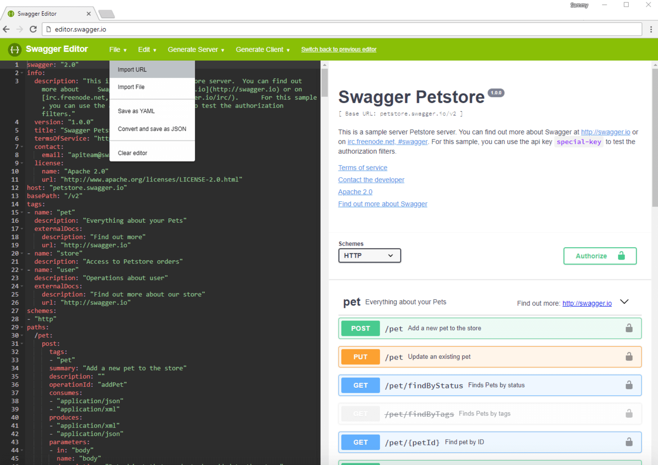
Navigate your web browser to http://editor.swagger.io/
. You should be welcomed with the following screen:
Here you’ll find a text editor containing the source code for the sample Swagger specification, and the human-readable API documentation on the right.
Let’s import the OpenFaaS Swagger specification. In the top menu, click on the File button, and then on Import URL:
You’ll see a pop-up, where you need to enter the address of the Swagger API specification. If you don’t see the pop-up, make sure pop-ups are enabled for your web browser.
In the field, enter the link to the Swagger OpenFaaS API specification: https://raw.githubusercontent.com/openfaas/faas/master/api-docs/swagger.yml
After clicking on the OK button, the Swagger editor will show you the API reference for OpenFaaS, which should look like this:
On the left side you can see the source of the API reference file, while on the right side you can see a list of endpoints, along with short descriptions. Clicking on an endpoint shows you more details about it, including what parameters it takes, what method it uses, and possible responses:
Once you know what endpoints are available and what parameters they expect, you can use them to manage your functions.
Next, you’ll use a curl
command to communicate with the API, so navigate back to your terminal. With the -u
flag, you will be able to pass the admin:your_openfaas_password
pair that you got in Step 3, while the -X
flag will define the request method. You will also pass your endpoint URL, https://example.com/system/functions
:
- curl -u admin:your_openfaas_password -X GET https://example.com/system/functions
You can see the required method for each endpoint in the API docs.
In Step 4, you deployed several sample functions, which should appear in the output:
Output[{"name":"base64","image":"functions/alpine:latest","invocationCount":0,"replicas":1,"envProcess":"base64","availableReplicas":0,"labels":{"com.openfaas.function":"base64","function":"true"}},{"name":"nodeinfo","image":"functions/nodeinfo:latest","invocationCount":0,"replicas":1,"envProcess":"","availableReplicas":0,"labels":{"com.openfaas.function":"nodeinfo","function":"true"}},{"name":"hubstats","image":"functions/hubstats:latest","invocationCount":0,"replicas":1,"envProcess":"","availableReplicas":0,"labels":{"com.openfaas.function":"hubstats","function":"true"}},{"name":"markdown","image":"functions/markdown-render:latest","invocationCount":0,"replicas":1,"envProcess":"","availableReplicas":0,"labels":{"com.openfaas.function":"markdown","function":"true"}},{"name":"echoit","image":"functions/alpine:latest","invocationCount":0,"replicas":1,"envProcess":"cat","availableReplicas":0,"labels":{"com.openfaas.function":"echoit","function":"true"}},{"name":"wordcount","image":"functions/alpine:latest","invocationCount":0,"replicas":1,"envProcess":"wc","availableReplicas":0,"labels":{"com.openfaas.function":"wordcount","function":"true"}}]
If you don’t see output that looks like this, or if you see an error, follow the on-screen instructions to resolve the problem before continuing with the tutorial. Make sure you’re sending the request to the correct endpoint using the recommended method and the right credentials. You can also check the logs for the gateway
service using the following command:
- docker service logs func_gateway
By default, the API response to the curl
call returns raw JSON without new lines, which is not human-readable. To parse it, pipe curl
’s response to the jq
utility, which will convert the JSON to human-readable form:
- curl -u admin:your_openfaas_password -X GET https://example.com/system/functions | jq
The output is now in human-readable form. You can see the function name, which you can use to manage and invoke functions with the API, the number of invocations, as well as information such as labels and number of replicas, relevant to Docker:
Output[
{
"name": "base64",
"image": "functions/alpine:latest",
"invocationCount": 0,
"replicas": 1,
"envProcess": "base64",
"availableReplicas": 0,
"labels": {
"com.openfaas.function": "base64",
"function": "true"
}
},
{
"name": "nodeinfo",
"image": "functions/nodeinfo:latest",
"invocationCount": 0,
"replicas": 1,
"envProcess": "",
"availableReplicas": 0,
"labels": {
"com.openfaas.function": "nodeinfo",
"function": "true"
}
},
{
"name": "hubstats",
"image": "functions/hubstats:latest",
"invocationCount": 0,
"replicas": 1,
"envProcess": "",
"availableReplicas": 0,
"labels": {
"com.openfaas.function": "hubstats",
"function": "true"
}
},
{
"name": "markdown",
"image": "functions/markdown-render:latest",
"invocationCount": 0,
"replicas": 1,
"envProcess": "",
"availableReplicas": 0,
"labels": {
"com.openfaas.function": "markdown",
"function": "true"
}
},
{
"name": "echoit",
"image": "functions/alpine:latest",
"invocationCount": 0,
"replicas": 1,
"envProcess": "cat",
"availableReplicas": 0,
"labels": {
"com.openfaas.function": "echoit",
"function": "true"
}
},
{
"name": "wordcount",
"image": "functions/alpine:latest",
"invocationCount": 0,
"replicas": 1,
"envProcess": "wc",
"availableReplicas": 0,
"labels": {
"com.openfaas.function": "wordcount",
"function": "true"
}
}
]
Let’s take one of these functions and execute it, using the API /function/function-name
endpoint. This endpoint is available over the POST method, where the -d
flag allows you to send data to the function.
For example, let’s run the following curl
command to execute the echoit
function, which comes with OpenFaaS out of the box and outputs the string you’ve sent it as a request. You can use the string "Sammy The Shark"
to demonstrate:
- curl -u admin:your_openfaas_password -X POST https://example.com/function/func_echoit -d "Sammy The Shark"
The output will show you Sammy The Shark
:
OutputSammy The Shark
If you see an error, follow the on-screen logs to resolve the problem before continuing with the tutorial. You can also check the gateway
service’s logs.
At this point, you’ve used the OpenFaaS API to manage and execute your functions. Let’s now take a look at the OpenFaaS Web UI.
OpenFaaS comes with a Web UI that you can use to add new and execute installed functions. In this step, you will install a function for generating QR Codes from the FaaS Store and generate a sample code.
To begin, point your web browser to https://example.com/ui/
. Note that the trailing slash is required to avoid a “not found” error.
In the HTTP authentication dialogue box, enter the username and password you got when deploying OpenFaaS in Step 3.
Once logged in, you will see available functions on the left side of the screen, along with the Deploy New Functions button used to install new functions.
Click on Deploy New Functions to deploy a new function. You will see the FaaS Store window, which provides community-tested functions that you can install with a single click:
In addition to these functions, you can also deploy functions manually from a Docker image.
For this tutorial, you will deploy the QR Code Generator function from the FaaS Store. Locate the QR Code Generator - Go item in the list, click on it, and then click the Deploy button at the bottom of the window:
After clicking Deploy, the Deploy A New Function window will close and the function will be deployed. In the list at the left side of the window you will see a listing for the qrcode-go
function. Click on this entry to select it. The main function window will show the function name, number of replicas, invocation count, and image, along with the option to invoke the function:
Let’s generate a QR code containing the URL with your domain. In the Request body field, type the content of the QR code you’d like to generate; in our case, this will be “example.com”. Once you’re done, click the Invoke button.
When you select either the Text or JSON output option, the function will output the file’s content, which is not usable or human-readable:
You can download a response. which in our case will be a PNG file with the QR code. To do this, select the Download option, and then click Invoke once again. Shortly after, you should have the QR code downloaded, which you can open with the image viewer of your choice:
In addition to deploying functions from the FaaS store or from Docker images, you can also create your own functions. In the next step, you will create a Python function using the FaaS command-line interface.
In the previous steps, you configured the FaaS CLI to work with your OpenFaaS server. The FaaS CLI is a command-line interface that you can use to manage OpenFaaS and install and run functions, just like you would over the API or using the Web UI.
Compared to the Web UI or the API, the FaaS CLI has templates for many programming languages that you can use to create your own functions. It can also build container images based on your function code and push images to an image registry, such as Docker Hub.
In this step, you will create a function, publish it to Docker Hub, and then run it on your OpenFaaS server. This function will be similar to the default echoit
function, which returns input passed as a request.
We will use Python to write our function. If you want to learn more about Python, you can check out our How To Code in Python 3 tutorial series and our How To Code in Python eBook.
Before creating the new function, let’s create a directory to store FaaS functions and navigate to it:
- mkdir ~/faas-functions
- cd ~/faas-functions
Execute the following command to create a new Python function called echo-input
. Make sure to replace your-docker-hub-username
with your Docker Hub username, as you’ll push the function to Docker Hub later:
- faas-cli new echo-input --lang python --prefix your-docker-hub-username --gateway https://example.com
The output contains confirmation about the successful function creation. If you don’t have templates downloaded, the CLI will download templates in your current directory:
Output2018/05/13 12:13:06 No templates found in current directory.
2018/05/13 12:13:06 Attempting to expand templates from https://github.com/openfaas/templates.git
2018/05/13 12:13:11 Fetched 12 template(s) : [csharp dockerfile go go-armhf node node-arm64 node-armhf python python-armhf python3 python3-armhf ruby] from https://github.com/openfaas/templates.git
Folder: echo-input created.
___ _____ ____
/ _ \ _ __ ___ _ __ | ___|_ _ __ _/ ___|
| | | | '_ \ / _ \ '_ \| |_ / _` |/ _` \___ \
| |_| | |_) | __/ | | | _| (_| | (_| |___) |
\___/| .__/ \___|_| |_|_| \__,_|\__,_|____/
|_|
Function created in folder: echo-input
Stack file written: echo-input.yml
The result of the faas-cli new
command is a newly-created ~/faas-fucntions/echo-input
directory containing the function’s code and the echo-input.yml
file. This file includes information about your function: what language it’s in, its name, and the server you will deploy it on.
Navigate to the ~/faas-fucntions/echo-input
directory:
- cd ~/faas-fucntions/echo-input
To see content of the directory, execute:
- ls
The directory contains two files: handler.py
, which contains the code for your function, and requirements.txt
, which contains the Python modules required by the function.
Since we don’t currently require any non-default Python modules, the requirements.txt
file is empty. You can check that by using the cat
command:
- cat requirements.txt
Next, let’s write a function that will return a request as a string.
The handler.py
file already has the sample handler code, which returns a received response as a string. Let’s take a look at the code:
- nano handler.py
The default function is called handle
and takes a single parameter, req
, that contains a request that’s passed to the function when it’s invoked. The function does only one thing, returning the passed request back as the response:
def handle(req):
"""handle a request to the function
Args:
req (str): request body
"""
return req
Let’s modify it to include additional text, replacing the string in the return
directive as follows:
return "Received message: " + req
Once you’re done, save the file and close your text editor.
Next, let’s build a Docker image from the function’s source code. Navigate to the faas-functions
directory where the echo-input.yml
file is located:
- cd ~/faas-functions
The following command builds the Docker image for your function:
- faas-cli build -f echo-input.yml
The output contains information about the build progress:
Output[0] > Building echo-input.
Clearing temporary build folder: ./build/echo-input/
Preparing ./echo-input/ ./build/echo-input/function
Building: sammy/echo-input with python template. Please wait..
Sending build context to Docker daemon 7.168kB
Step 1/16 : FROM python:2.7-alpine
---> 5fdd069daf25
Step 2/16 : RUN apk --no-cache add curl && echo "Pulling watchdog binary from Github." && curl -sSL https://github.com/openfaas/faas/releases/download/0.8.0/fwatchdog > /usr/bin/fwatchdog && chmod +x /usr/bin/fwatchdog && apk del curl --no-cache
---> Using cache
---> 247d4772623a
Step 3/16 : WORKDIR /root/
---> Using cache
---> 532cc683d67b
Step 4/16 : COPY index.py .
---> Using cache
---> b4b512152257
Step 5/16 : COPY requirements.txt .
---> Using cache
---> 3f9cbb311ab4
Step 6/16 : RUN pip install -r requirements.txt
---> Using cache
---> dd7415c792b1
Step 7/16 : RUN mkdir -p function
---> Using cache
---> 96c25051cefc
Step 8/16 : RUN touch ./function/__init__.py
---> Using cache
---> 77a9db274e32
Step 9/16 : WORKDIR /root/function/
---> Using cache
---> 88a876eca9e3
Step 10/16 : COPY function/requirements.txt .
---> Using cache
---> f9ba5effdc5a
Step 11/16 : RUN pip install -r requirements.txt
---> Using cache
---> 394a1dd9e4d7
Step 12/16 : WORKDIR /root/
---> Using cache
---> 5a5893c25b65
Step 13/16 : COPY function function
---> eeddfa67018d
Step 14/16 : ENV fprocess="python index.py"
---> Running in 8e53df4583f2
Removing intermediate container 8e53df4583f2
---> fb5086bc7f6c
Step 15/16 : HEALTHCHECK --interval=1s CMD [ -e /tmp/.lock ] || exit 1
---> Running in b38681a71378
Removing intermediate container b38681a71378
---> b04c045b0994
Step 16/16 : CMD ["fwatchdog"]
---> Running in c5a11078df3d
Removing intermediate container c5a11078df3d
---> bc5f08157c5a
Successfully built bc5f08157c5a
Successfully tagged sammy/echo-input:latest
Image: your-docker-hub-username/echo-input built.
[0] < Building echo-input done.
[0] worker done.
If you get an error, make sure to resolve it by following the on-screen instructions before deploying the function.
You will need to containerize your OpenFaaS function in order to deploy it. Containerizing applications ensures that the environment needed to run your application can be easily reproduced, and your application can be easily deployed, scaled, and updated.
For this tutorial, we’ll use Docker Hub, as it’s a free solution, but you can use any container registry, including your own private registry.
Run the following command to push the image you built to your specified repository on Docker Hub:
- faas-cli push -f echo-input.yml
Pushing will take several minutes, depending on your internet connection speed. The output contains the image’s upload progress:
Output[0] > Pushing echo-input.
The push refers to repository [docker.io/sammy/echo-input]
320ea573b385: Pushed
9d87e56f5d0c: Pushed
6f79b75e7434: Pushed
23aac2d8ecf2: Pushed
2bec17d09b7e: Pushed
e5a0e5ab3be6: Pushed
e9c8ca932f1b: Pushed
beae1d55b4ce: Pushed
2fcae03ed1f7: Pushed
62103d5daa03: Mounted from library/python
f6ac6def937b: Mounted from library/python
55c108c7613c: Mounted from library/python
e53f74215d12: Mounted from library/python
latest: digest: sha256:794fa942c2f593286370bbab2b6c6b75b9c4dcde84f62f522e59fb0f52ba05c1 size: 3033
[0] < Pushing echo-input done.
[0] worker done.
Finally, with your image pushed to Docker Hub, you can use it to deploy a function to your OpenFaaS server.
To deploy your function, run the deploy
command, which takes the path to the manifest that describes your function, as well as the address of your OpenFaaS server:
- faas-cli deploy -f echo-input.yml --gateway https://example.com
The output shows the status of the deployment, along with the name of the function you’re deploying and the deployment status code:
OutputDeploying: echo-input.
Deployed. 200 OK.
URL: https://example.com/function/echo-input
If the deployment is successful, you will see a 200
status code. In the case of errors, follow the provided instructions to fix the problem before continuing.
At this point your function is deployed and ready to be used. You can test that it is working as expected by invoking it.
To invoke a function with the FaaS CLI, use the invoke
command by passing the function name and OpenFaaS address to it. After executing the command, you’ll be asked to enter the request you want to send to the function.
Execute the following command to invoke the echo-input
function:
- faas-cli invoke echo-input --gateway https://example.com
You’ll be asked to enter the request you want to send to the function:
OutputReading from STDIN - hit (Control + D) to stop.
Enter the text you want to send to the function, such as:
Sammy The Shark!
Once you’re done, press ENTER
and then CTRL + D
to finish the request. The CTRL + D
shortcut in the terminal is used to register an End-of-File (EOF). The OpenFaaS CLI stops reading from the terminal once EOF is received.
After several seconds, the command will output the function’s response:
OutputReading from STDIN - hit (Control + D) to stop.
Sammy The Shark!
Received message: Sammy The Shark!
If you don’t see the output or you get an error, retrace the preceding steps to make sure you’ve deployed the function as explained and follow the on-screen instructions to resolve the problem.
At this point, you’ve interacted with your function using three methods: the Web UI, the API, and the CLI. Being able to execute your functions with any of these methods offers you the flexibility of deciding how you would like to integrate functions into your existing workflows.
In this tutorial, you’ve used serverless architecture and OpenFaaS to deploy and manage your applications using the OpenFaaS API, Web UI, and CLI. You also secured your infrastructure by leveraging Traefik to provide SSL using Let’s Encrypt.
If you want to learn more about the OpenFaaS project, you can check out their website and the project’s official documentation.
]]>Tried contacting support but no satisfactory answer. they gave me 2 link as below, I tried and couldn’t find anything. https://unix.stackexchange.com/questions/70538/grub-error-file-grub-i386-pc-normal-mod-not-found https://askubuntu.com/questions/266429/error-file-grub-i386-pc-normal-mod-not-found
The above links suggested to change the prefix I tried, but it didn’t worked, here is the output of ls. grub rescue> ls (hd0,gpt1)/boot ./ …/ efi/ grub rescue> ls (hd0,gpt1)/boot/efi ./ …/ NO FILES/FOLDER inside efi folder and there no grub folder as well. So I think grub is removed. And I have no idea why/how.
SOME INFO ON WHY & HOW PROBLEM STARTED:
Please help me out. Everything is down.
]]>This article supplements a webinar series on deploying and managing containerized workloads in the cloud. The series covers the essentials of containers, including managing container lifecycles, deploying multi-container applications, scaling workloads, and working with Kubernetes. It also highlights best practices for running stateful applications.
This tutorial includes the concepts and commands in the fifth session of the series, Deploying and Scaling Microservices in Kubernetes.
Kubernetes is an open-source container orchestration tool for managing containerized applications. In the previous tutorial in this series, A Closer Look at Kubernetes you learned the building blocks of Kubernetes.
In this tutorial, you will apply the concepts from the previous tutorials to build, deploy, and manage an end-to-end microservices application in Kubernetes. The sample web application you’ll use in this tutorial is a “todo list” application written in Node.js that uses MongoDB as a database. This is the same application we used in the tutorial Building Containerized Applications.
You’ll build a container image for this app from a Dockerfile, push the image to Docker Hub, and then deploy it to your cluster. Then you’ll scale the app to meet increased demand.
To complete this tutorial, you’ll need:
A Kubernetes cluster, which you can configure in the third part of this tutorial series, Getting Started with Kubernetes.
An active Docker Hub account to store the image.
Git installed on your local machine. You can follow the tutorial Contributing to Open Source: Getting Started with Git to install and set up Git on your computer.
We will begin by containerizing the web application by packaging it into a Docker image.
Start by changing to your home directory, then use Git to clone this tutorial’s sample web application from its official repository on GitHub.
- cd ~
- git clone https://github.com/janakiramm/todo-app.git
Build the container image from the Dockerfile. Use the -t switch to tag the image with the registry username, image name, and an optional tag.
- docker build -t sammy/todo .
The output confirms that the image was successfully built and tagged appropriately.
OutputSending build context to Docker daemon 8.238MB
Step 1/7 : FROM node:slim
---> 286b1e0e7d3f
Step 2/7 : LABEL maintainer = "jani@janakiram.com"
---> Using cache
---> ab0e049cf6f8
Step 3/7 : RUN mkdir -p /usr/src/app
---> Using cache
---> 897176832f4d
Step 4/7 : WORKDIR /usr/src/app
---> Using cache
---> 3670f0147bed
Step 5/7 : COPY ./app/ ./
---> Using cache
---> e28c7c1be1a0
Step 6/7 : RUN npm install
---> Using cache
---> 7ce5b1d0aa65
Step 7/7 : CMD node app.js
---> Using cache
---> 2cef2238de24
Successfully built 2cef2238de24
Successfully tagged sammy/todo-app:latest
Verify that the image is created by running the docker images command.
- docker images
You can see the size of the image along with the time since it was created.
OutputREPOSITORY TAG IMAGE ID CREATED SIZE
sammy/todo-app latest 81f5f605d1ca 9 minutes ago 236MB
Next, push your image to the public registry on Docker Hub. To do this, log in to your Docker Hub account:
- docker login
Once you provide your credentials, tag your image using your Docker Hub username:
- docker tag your_docker_hub_username/todo-app
Then push your image to Docker Hub:
- docker push
You can verify that the new image is available by searching Docker Hub in your web browser.
With the Docker image pushed to the registry, let’s package the application for Kubernetes.
The application uses MongoDB to store to-do lists created through the web application. To run MongoDB in Kubernetes, we need to package it as a Pod. When we launch this Pod, it will run a single instance of MongoDB.
Create a new YAML file called db-pod.yaml:
- nano db-pod.yaml
Add the following code which defines a Pod with one container based on MongoDB. We expose port 27017
, the standard port used by MongoDB. Notice that the definition contains the labels name
and app
. We’ll use those labels to identify and configure specific Pods.
apiVersion: v1
kind: Pod
metadata:
name: db
labels:
name: mongo
app: todoapp
spec:
containers:
- image: mongo
name: mongo
ports:
- name: mongo
containerPort: 27017
volumeMounts:
- name: mongo-storage
mountPath: /data/db
volumes:
- name: mongo-storage
hostPath:
path: /data/db
The data is stored in the volume called mongo-storage
which is mapped to the /data/db
location of the node. For more information on Volumes, refer to the official Kubernetes volumes documentation.
Run the following command to create a Pod.
- kubectl create -f db-pod.yml
You’ll see this output:
Outputpod "db" created
Now verify the creation of the Pod.
- kubectl get pods
The output shows the Pod and indicates that it is running:
OutputNAME READY STATUS RESTARTS AGE
db 1/1 Running 0 2m
Let’s make this Pod accessible to the internal consumers of the cluster.
Create a new file called db-service.yaml
that contains this code which defines the Service for MongoDB:
apiVersion: v1
kind: Service
metadata:
name: db
labels:
name: mongo
app: todoapp
spec:
selector:
name: mongo
type: ClusterIP
ports:
- name: db
port: 27017
targetPort: 27017
The Service discovers all the Pods in the same Namespace that match the Label with name: db
. The selector
section of the YAML file explicitly defines this association.
We specify that the Service is visible within the cluster through the declaration type: ClusterIP
.
Save the file and exit the editor. Then use kubectl
to submit it to the cluster.
- kubectl create -f db-service.yml
You’ll see this output indicating the Service was created successfully:
Outputservice "db" created
Let’s get the port on which the Pod is available.
- kubectl get services
You’ll see this output:
OutputNAME TYPE CLUSTER-IP EXTERNAL-IP PORT(S) AGE
db ClusterIP 10.109.114.243 <none> 27017/TCP 14s
kubernetes ClusterIP 10.96.0.1 <none> 443/TCP 47m
From this output, you can see that the Service is available on port 27017
. The web application can reach MongoDB through this service. When it uses the hostname db
, the DNS service running within Kubernetes will resolve the address to the ClusterIP associated with the Service. This mechanism allows Pods to discover and communicate with each other.
With the database Pod and Service in place, let’s create a Pod for the web application.
Let’s package the Docker image you created in the first step of this tutorial as a Pod and deploy it to the cluster. This will act as the front-end web application layer accessible to end users.
Create a new YAML file called web-pod.yaml
:
- nano web-pod.yaml
Add the following code which defines a Pod with one container based on the sammy/todo-app
Docker image. It is exposed on port 3000
over the TCP protocol.
apiVersion: v1
kind: Pod
metadata:
name: web
labels:
name: web
app: todoapp
spec:
containers:
- image: sammy/todo-app
name: myweb
ports:
- containerPort: 3000
Notice that the definition contains the labels name
and app
. A Service will use these labels to route inbound traffic to the appropriate ports.
Run the following command to create the Pod:
- kubectl create -f web-pod.yaml
Outputpod "web" created
Let’s verify the creation of the Pod:
- kubectl get pods
OutputNAME READY STATUS RESTARTS AGE
db 1/1 Running 0 8m
web 1/1 Running 0 9s
Notice that we have both the MongoDB database and web app running as Pods.
Now we will make the web
Pod accessible to the public Internet.
Services expose a set of Pods either internally or externally. Let’s define a Service that makes the web
Pod publicly available. We’ll expose it through a NodePort, a scheme that makes the Pod accessible through an arbitrary port opened on each Node of the cluster.
Create a new file called web-service.yaml
that contains this code which defines the Service for the app:
apiVersion: v1
kind: Service
metadata:
name: web
labels:
name: web
app: todoapp
spec:
selector:
name: web
type: NodePort
ports:
- name: http
port: 3000
targetPort: 3000
protocol: TCP
The Service discovers all the Pods in the same Namespace that match the Label with the name web
. The selector section of the YAML file explicitly defines this association.
We specify that the Service is of type NodePort
through the type: NodePort
declaration.
Use kubectl
to submit this to the cluster.
- kubectl create -f web-service.yml
You’ll see this output indicating the Service was created successfully:
Outputservice "web" created
Let’s get the port on which the Pod is available.
- kubectl get services
OutputNAME TYPE CLUSTER-IP EXTERNAL-IP PORT(S) AGE
db ClusterIP 10.109.114.243 <none> 27017/TCP 12m
kubernetes ClusterIP 10.96.0.1 <none> 443/TCP 59m
web NodePort 10.107.206.92 <none> 3000:30770/TCP 12s
From this output, we see that the Service is available on port 30770
. Let’s try to connect to one of the Worker Nodes.
Obtain the public IP address for one of the Worker Nodes associated with your Kubernetes Cluster by using the DigitalOcean console.
Once you’ve obtained the IP address, use the curl
command to make an HTTP request to one of the nodes on port 30770
:
- curl http://your_worker_ip_address:30770
You’ll see output similar to this:
Output<!DOCTYPE html>
<html>
<head>
<title>Containers Todo Example</title>
<link rel='stylesheet' href='/stylesheets/screen.css' />
<!--[if lt IE 9]>
<script src="http://html5shiv.googlecode.com/svn/trunk/html5.js"></script>
<![endif]-->
</head>
<body>
<div id="layout">
<h1 id="page-title">Containers Todo Example</h1>
<div id="list">
<form action="/create" method="post" accept-charset="utf-8">
<div class="item-new">
<input class="input" type="text" name="content" />
</div>
</form>
</div>
<div id="layout-footer"></div>
</div>
<script src="/javascripts/ga.js"></script>
</body>
</html>
You’ve defined the web Pod and a Service. Now let’s look at scaling it with Replica Sets.
A Replica Set ensures that a minimum number of Pods are running in the cluster at all times. When a Pod is packaged as a Replica Set, Kubernetes will always run the minimum number of Pods defined in the specification.
Let’s delete the current Pod and recreate two Pods through the Replica Set. If we leave the Pod running it will not be a part of the Replica Set. Thus, it’s a good idea to launch Pods through a Replica Set, even when the count is just one.
First, delete the existing Pod.
- kubectl delete pod web
Outputpod "web" deleted
Now create a new Replica Set declaration. The definition of the Replica Set is identical to a Pod. The key difference is that it contains the replica
element which defines the number of Pods that need to run. Like a Pod, it also contains Labels as metadata that help in Service discovery.
Create the file web-rs.yaml
and add this code to the file:
apiVersion: extensions/v1beta1
kind: ReplicaSet
metadata:
name: web
labels:
name: web
app: todoapp
spec:
replicas: 2
template:
metadata:
labels:
name: web
spec:
containers:
- name: web
image: sammy/todo-app
ports:
- containerPort: 3000
Save and close the file.
Now create the Replica Set:
- kubectl create -f web-rs.yaml
Outputreplicaset "web" created
Then check the number of Pods:
- kubectl get pods
OutputNAME READY STATUS RESTARTS AGE
db 1/1 Running 0 18m
web-n5l5h 1/1 Running 0 25s
web-wh6nf 1/1 Running 0 25s
When we access the Service through the NodePort, the request will be sent to one of the Pods managed by the Replica Set.
Let’s test the functionality of a Replica Set by deleting one of the Pods and seeing what happens:
- kubectl delete pod web-wh6nf
Outputpod "web-wh6nf" deleted
Look at the Pods again:
- kubectl get pods
OutputNAME READY STATUS RESTARTS AGE
db 1/1 Running 0 19m
web-n5l5h 1/1 Running 0 1m
web-wh6nf 1/1 Terminating 0 1m
web-ws59m 0/1 ContainerCreating 0 2s
As soon as the Pod is deleted, Kubernetes has created another one to ensure the desired count is maintained.
We can scale the Replica Set to run additional web Pods.
Run the following command to scale the web application to 10 Pods.
- kubectl scale rs/web --replicas=10
Outputreplicaset "web" scaled
Check the Pod count:
- kubectl get pods
You’ll see this output:
OutputNAME READY STATUS RESTARTS AGE
db 1/1 Running 0 22m
web-4nh4g 1/1 Running 0 21s
web-7vbb5 1/1 Running 0 21s
web-8zd55 1/1 Running 0 21s
web-f8hvq 0/1 ContainerCreating 0 21s
web-ffrt6 1/1 Running 0 21s
web-k6zv7 0/1 ContainerCreating 0 21s
web-n5l5h 1/1 Running 0 3m
web-qmdxn 1/1 Running 0 21s
web-vc45m 1/1 Running 0 21s
web-ws59m 1/1 Running 0 2m
Kubernetes has initiated the process of scaling the web
Pod. When the request comes to the Service via the NodePort, it gets routed to one of the Pods in the Replica Set.
When the traffic and load subsides, we can revert to the original configuration of two Pods.
kubectl scale rs/web --replicas=2
Outputreplicaset "web" scaled
This command terminates all the Pods except two.
- kubectl get pods
OutputNAME READY STATUS RESTARTS AGE
db 1/1 Running 0 24m
web-4nh4g 1/1 Terminating 0 2m
web-7vbb5 1/1 Terminating 0 2m
web-8zd55 1/1 Terminating 0 2m
web-f8hvq 1/1 Terminating 0 2m
web-ffrt6 1/1 Terminating 0 2m
web-k6zv7 1/1 Terminating 0 2m
web-n5l5h 1/1 Running 0 5m
web-qmdxn 1/1 Terminating 0 2m
web-vc45m 1/1 Terminating 0 2m
web-ws59m 1/1 Running 0 4m
To verify the availability of the Replica Set, try deleting one of the Pods and check the count.
- kubectl delete pod web-ws59m
Outputpod "web-ws59m" deleted
- kubectl get pods
OutputNAME READY STATUS RESTARTS AGE
db 1/1 Running 0 25m
web-n5l5h 1/1 Running 0 7m
web-ws59m 1/1 Terminating 0 5m
web-z6r2g 0/1 ContainerCreating 0 5s
As soon as the Pod count changes, Kubernetes adjusts it to match the count defined in the YAML file. When one of the web Pods in the Replica Set is deleted, another Pod is immediately created to maintain the desired count. This ensures high availability of the application by ensuring that the minimum number of Pods are running all the time.
You can delete all the objects created during this tutorial with the following command:
- kubectl delete -f db-pod.yaml -f db-service.yaml -f web-rs.yaml -f web-service.yaml
Outputpod "db" deleted
service "db" deleted
replicaset "web" deleted
service "web" deleted
In this tutorial, you applied all the concepts covered in the series to package, deploy, and scale a microservices applications.
In the next part of this series, you will learn how to make MongoDB highly available by running it as a StatefulSet.
]]>System and infrastructure monitoring is a core responsibility of operations teams of all sizes. The industry has collectively developed many strategies and tools to help monitor servers, collect important data, and respond to incidents and changing conditions in varying environments. However, as software methodologies and infrastructure designs evolve, monitoring must adapt to meet new challenges and provide insight in relatively unfamiliar territory.
So far in this series, we’ve discussed what metrics, monitoring, and alerting are and the qualities of good monitoring systems. We talked about gathering metrics from your infrastructure and applications and the important signals to monitor throughout your infrastructure. In our last guide, we covered how to put metrics and alerting into practice by understanding individual components and the qualities of good alert design.
In this guide, we will take a look at how monitoring and metrics collection changes for highly distributed architectures and microservices. The growing popularity of cloud computing, big data clusters, and instance orchestration layers has forced operations professionals to rethink how to design monitoring at scale and tackle unique problems with better instrumentation. We will talk about what makes new models of deployment different and what strategies can be used to meet these new demands.
In order to model and mirror the systems it watches, monitoring infrastructure has always been somewhat distributed. However, many modern development practices—including designs around microservices, containers, and interchangeable, ephemeral compute instances—have changed the monitoring landscape dramatically. In many cases, the core features of these advancements are the very factors that make monitoring most difficult. Let’s take a moment to look at some of the ways these differ from traditional environments and how that affects monitoring.
Some of the most fundamental changes in the way many systems behave are due to an explosion in new abstraction layers that software can be designed around. Container technology has changed the relationship between deployed software and the underlying operating system. Applications deployed in containers have different relationship to the outside world, other programs, and the host operating system than applications deployed through conventional means. Kernel and network abstractions can lead to different understandings of the operating environment depending on which layer you check.
This level of abstraction is incredibly helpful in many ways by creating consistent deployment strategies, making it easier to migrate work between hosts, and allowing developers close control over their applications’ runtime environments. However, these new capabilities come at the expense of increased complexity and a more distant relationship with the resources powering each process.
One commonality among newer paradigms is an increased reliance on internal network communication to coordinate and accomplish tasks. What was formerly the domain of a single application might now be spread among many components that need to coordinate and share information. This has a few repercussions in terms of communication infrastructure and monitoring.
First, because these models are built upon communication between small, discrete services, network health becomes more important than ever. In traditional, more monolithic architectures, coordinating tasks, sharing information, and organizing results was largely accomplished within applications with regular programming logic or through a comparably small amount of external communication. In contrast, the logical flow of highly distributed applications use the network to synchronize, check the health of peers, and pass information. Network health and performance directly impacts more functionality than previously, which means more intensive monitoring is needed to guarantee correct operation.
While the network has become more critical than ever, the ability to effectively monitor it is increasingly challenging due to the extended number of participants and individual lines of communication. Instead of tracking interactions between a few applications, correct communication between dozens, hundreds, or thousands of different points becomes necessary to ensure the same functionality. In addition to considerations of complexity, the increased volume of traffic also puts additional strain on the networking resources available, further compounding the necessity of reliable monitoring.
Above, we mentioned in passing the tendency for modern architectures to divide up work and functionality between many smaller, discrete components. These designs can have a direct impact on the monitoring landscape because they make clarity and comprehensibility especially valuable but increasingly elusive.
More robust tooling and instrumentation is required to ensure good working order. However, because the responsibility for completing any given task is fragmented and split between different workers (potentially on many different physical hosts), understanding where responsibility lies for performance issues or errors can be difficult. Requests and units of work that touch dozens of components, many of which are selected from pools of possible candidates, can make request path visualization or root cause analysis impractical using traditional mechanisms.
A further struggle in adapting conventional monitoring is tracking short-lived or ephemeral units sensibly. Whether the units of concern are cloud compute instances, container instances, or other abstractions, these components often violate some of the assumptions made by conventional monitoring software.
For instance, in order to distinguish between a problematic downed node and an instance that was intentionally destroyed to scale down, the monitoring system must have a more intimate understanding of your provisioning and management layer than was previously necessary. For many modern systems, these events happen a great deal more frequently, so manually adjusting the monitoring domain each time is not practical. The deployment environment shifts more rapidly with these designs, so the monitoring layer must adopt new strategies to remain valuable.
One question that many systems must face is what to do with the data from destroyed instances. While work units may be provisioned and deprovisioned rapidly to accommodate changing demands, a decision must be made about what to do with the data related to the old instances. Data doesn’t necessarily lose its value immediately just because the underlying worker is no longer available. When hundreds or thousands of nodes might come and go each day, it can be difficult to know how to best construct a narrative about the overall operational health of your system from the fragmented data of short-lived instances.
Now that we’ve identified some of the unique challenges of distributed architectures and microservices, we can talk about ways monitoring systems can work within these realities. Some of the solutions involve re-evaluating and isolating what is most valuable about different types of metrics, while others involve new tooling or new ways of understanding the environment they inhabit.
The increase in total traffic volume caused by the elevated number of services is one of the most straightforward problems to think about. Beyond the swell in transfer numbers caused by new architectures, monitoring activity itself can start to bog down the network and steal host resources. To best deal with increased volume, you can either scale out your monitoring infrastructure or reduce the resolution of the data you work with. Both approaches are worth looking at, but we will focus on the second one as it represents a more extensible and broadly useful solution.
Changing your data sampling rates can minimize the amount of data your system needs to collect from hosts. Sampling is a normal part of metrics collection that represents how frequently you ask for new values for a metric. Increasing the sampling interval will reduce the amount of data you have to handle but also reduce the resolution—the level of detail—of your data. While you must be careful and understand your minimum useful resolution, tweaking the data collection rates can have a profound impact on how many monitoring clients your system can adequately serve.
To decrease the loss of information resulting from lower resolutions, one option is to continue to collect data on hosts at the same frequency, but compile it into more digestible numbers for transfer over the network. Individual computers can aggregate and average metric values and send summaries to the monitoring system. This can help reduce the network traffic while maintaining accuracy since a large number of data points are still taken into account. Note that this helps reduce the data collection’s influence on the network, but does not by itself help with strain involved with gathering those numbers within the host.
As mentioned above, one of the major differentiators between traditional systems and modern architectures is the break down of what components participate in handling requests. In distributed systems and microservices, a unit of work is much more likely to be given to a pool of workers through some type of scheduling or arbitrating layer. This has implications on many of the automated processes you might build around monitoring.
In environments that use pools of interchangeable workers, health checking and alert policies can grow to have complex relationships with the infrastructure they monitor. Health checks on individual workers can be useful to automatically decommission and recycle defective units. However if you have automation in place, at scale, it doesn’t matter much if a single web server fails out of a large pool. The system will self-correct to make sure only healthy units are in the active pool receiving requests.
Though host health checks can catch defective units, health checking the pool itself is more appropriate for alerting. The pool’s ability to satisfy the current workload has greater bearing on user experience than the capabilities of any individual worker. Alerts based on the number of healthy members, latency for the pool aggregate, or the pool error rate can notify operators of problems that are more difficult to automatically mitigate and more likely to impact users.
In general, the monitoring layer in distributed systems needs to have a more complete understanding of the deployment environment and the provisioning mechanisms. Automated life cycle management becomes incredibly valuable because of the number of individual units involved in these architectures. Regardless of whether the units are raw containers, containers within an orchestration framework, or compute nodes in a cloud environment, a management layer exists that exposes health information and accepts commands to scale and respond to events.
The number of pieces in play increases the statistical likelihood of failure. With all other factors being equal, this would require more human intervention to respond to and mitigate these issues. Since the monitoring system is responsible for identifying failures and service degradation, if it can hook into the platform’s control interfaces, it can alleviate a large class of these problems. An immediate and automatic response triggered by the monitoring software can help maintain your system’s operational health.
This close relationship between the monitoring system and the deployment platform is not necessarily required or common in other architectures. But automated distributed systems aim to be self-regulating, with the ability to scale and adjust based on preconfigured rules and observed status. The monitoring system in this case takes on a central role in controlling the environment and deciding when to take action.
Another reason the monitoring system must have knowledge of the provisioning layer is to deal with the side effects of ephemeral instances. In environments where there is frequent turnover in the working instances, the monitoring system depends on information from a side channel to understand when actions were intentional or not. For instance, systems that can read API events from a provisioner can react differently when a server is destroyed intentionally by an operator than when a server suddenly becomes unresponsive with no associated event. Being able to differentiate between these events can help your monitoring remain useful, accurate, and trustworthy even though the underlying infrastructure might change frequently.
One of the most challenging aspects of highly distributed workloads is understanding the interplay between different components and isolating responsibility when attempting root cause analysis. Since a single request might touch dozens of small programs to generate a response, it can be difficult to interpret where bottlenecks or performance changes originate. To provide better information about how each component contributes to latency and processing overhead, a technique called distributed tracing has emerged.
Distributed tracing is an approach to instrumenting systems that works by adding code to each component to illuminate the request processing as it traverses your services. Each request is given a unique identifier at the edge of your infrastructure that is passed along as the task traverses your infrastructure. Each service then uses this ID to report errors and the timestamps for when it first saw the request and when it handed it off to the next stage. By aggregating the reports from components using the request ID, a detailed path with accurate timing data can be traced through your infrastructure.
This method can be used to understand how much time is spent on each part of a process and clearly identify any serious increases in latency. This extra instrumentation is a way to adapt metrics collection to large numbers of processing components. When mapped visually with time on the x axis, the resulting display shows the relationship between different stages, how long each process ran, and the dependency relationship between events that must run in parallel. This can be incredibly useful in understanding how to improve your systems and how time is being spent.
We’ve discussed how distributed architectures can make root cause analysis and operational clarity difficult to achieve. In many cases, changing the way that humans respond to and investigate issues is part of the answer to these ambiguities. Setting tools up to expose information in a way that empowers you to analyze the situation methodically can help sort through the many layers of data available. In this section, we’ll discuss ways to set yourself up for success when troubleshooting issues in large, distributed environments.
The first step to ensure you can respond to problems in your systems is to know when they are occurring. In our guide on gathering metrics from your infrastructure and applications, we introduced the four golden signals—monitoring indicators identified by the Google SRE team as the most vital to track. The four signals are:
These are still the best places to start when instrumenting your systems, but the number of layers that must be watched usually increases for highly distributed systems. The underlying infrastructure, the orchestration plane, and the working layer each need robust monitoring with thoughtful alerts set to identify important changes. The alerting conditions may grow in complexity to account for the ephemeral elements inherent within the platform.
Once your systems have identified an anomaly and notified your staff, your team needs to begin gathering data. Before continuing on from this step, they should have an understanding of what components are affected, when the incident began, and what specific alert condition was triggered.
The most useful way to begin understanding the scope of an incident is to start at a high level. Begin investigating by checking dashboards and visualizations that gather and generalize information from across your systems. This can help you quickly identify correlated factors and understand the immediate user-facing impact. During this process, you should be able to overlay information from different components and hosts.
The goal of this stage is to begin to create a mental or physical inventory of items to check in more detail and to start to prioritize your investigation. If you can identify a chain of related issues that traverse different layers, the lowest layer should take precedence: fixes to foundational layers often resolve symptoms at higher levels. The list of affected systems can serve as an informal checklist of places to validate fixes against later when mitigation is deployed.
Once you feel that you have a reasonable high level view of the incident, drill down for more details into the components and systems on your list in order of priority. Detailed metrics about individual units will help you trace the route of the failure to the lowest responsible resource. While looking at more fine-grained dashboards and log entries, reference the list of affected components to try to further understand how side effects are being propagated through the system. With microservices, the number of interdependent components means that problems spill over to other services more frequently.
This stage is focused on isolating the service, component, or system responsible for the initial incident and identifying what specific problem is occurring. This might be newly deployed code, faulty physical infrastructure, a mistake or bug in the orchestration layer, or a change in workload that the system could not handle gracefully. Diagnosing what is happening and why allows you to discover how to mitigate the issue and regain operational health. Understanding the extent to which resolving this issue might fix issues reported on other systems can help you continue to prioritize mitigation tasks.
Once the specifics are identified, you can work on resolving or mitigating the problem. In many cases, there might be an obvious, quick way to restore service by either providing more resources, rolling back, or rerouting traffic to an alternative implementation. In these scenarios, resolution will be broken into three phases:
In many distributed systems, redundancy and highly available components will ensure that service is restored quickly, though more work might be necessary in the background to restore redundancy or bring the system out of a degraded state. You should use the list of impacted components compiled earlier as a measuring stick to determine whether your initial mitigation resolves cascading service issues. As the sophistication of the monitoring systems evolves, it may also be able to automate some of these fuller recovery processes by sending commands to the provisioning layer to bring up new instances of failed units or cycle out misbehaving units.
Given the automation possible in the first two phases, the most important work for the operations team is often understanding the root causes of an event. The knowledge gleaned from this process can be used to develop new triggers and policies to help predict future occurrences and further automate the system’s reactions. The monitoring software often gains new capabilities in response to each incident to guard against the newly discovered failure scenarios. For distributed systems, distributed traces, log entries, time series visualizations, and events like recent deploys can help you reconstruct the sequence of events and identify where software and human processes could be improved.
Because of the particular complexity inherent in large distributed systems, it is important to treat the resolution process of any significant event as an opportunity to learn and fine-tune your systems. The number of separate components and communication paths involved forces heavy reliance on automation and tools to help manage complexity. Encoding new lessons into the response mechanisms and rule sets of these components (as well as operational policies your team abides by) is the best way for your monitoring system to keep the management footprint for your team in check.
In this guide, we’ve talked about some of the specific challenges that distributed architectures and microservice designs can introduce for monitoring and visibility software. Modern ways of building systems break some assumptions of traditional methods, requiring different approaches to handle the new configuration environments. We explored the adjustments you’ll need to consider as you move from monolithic systems to those that increasingly depend on ephemeral, cloud or container-based workers and high volume network coordination. Afterwards, we discussed some ways that your system architecture might affect the way you respond to incidents and resolution.
]]>