Tutorial
A Guide to Time Series Forecasting with Prophet in Python 3

Introduction
In previous tutorials, we showed how to visualize and manipulate time series data, and how to leverage the ARIMA method to produce forecasts from time series data. We noted how the correct parametrization of ARIMA models could be a complicated manual process that required a certain amount of time.
Other statistical programming languages such a R provide automated ways to solve this issue, but those have yet to be officially ported over to Python. Fortunately, the Core Data Science team at Facebook recently published a new method called Prophet, which enables data analysts and developers alike to perform forecasting at scale in Python 3.
Prerequisites
This guide will cover how to do time series analysis on either a local desktop or a remote server. Working with large datasets can be memory intensive, so in either case, the computer will need at least 2GB of memory to perform some of the calculations in this guide.
For this tutorial, we’ll be using Jupyter Notebook to work with the data. If you do not have it already, you should follow our tutorial to install and set up Jupyter Notebook for Python 3.
Step 1 — Pull Dataset and Install Packages
To set up our environment for time series forecasting with Prophet, let’s first move into our local programming environment or server-based programming environment:
- cd environments
- . my_env/bin/activate
From here, let’s create a new directory for our project. We will call it timeseries and then move into the directory. If you call the project a different name, be sure to substitute your name for timeseries throughout the guide:
- mkdir timeseries
- cd timeseries
We’ll be working with the Box and Jenkins (1976) Airline Passengers dataset, which contains time series data on the monthly number of airline passengers between 1949 and 1960. You can save the data by using the curl command with the -O flag to write output to a file and download the CSV:
curl -O https://assets.digitalocean.com/articles/eng_python/prophet/AirPassengers.csv
This tutorial will require the pandas, matplotlib, numpy, cython and fbprophet libraries. Like most other Python packages, we can install the pandas, numpy, cython and matplotlib libraries with pip:
pip install pandas matplotlib numpy cython
In order to compute its forecasts, the fbprophet library relies on the STAN programming language, named in honor of the mathematician Stanislaw Ulam. Before installing fbprophet, we therefore need to make sure that the pystan Python wrapper to STAN is installed:
pip install pystan
Once this is done we can install Prophet by using pip:
pip install fbprophet
Now that we are all set up, we can start working with the installed packages.
Step 2 — Import Packages and Load Data
To begin working with our data, we will start up Jupyter Notebook:
- jupyter notebook
To create a new notebook file, select New > Python 3 from the top right pull-down menu:
This will open a notebook which allows us to load the required libraries.
As is best practice, start by importing the libraries you will need at the top of your notebook (notice the standard shorthands used to reference pandas, matplotlib and statsmodels):
%matplotlib inline
import pandas as pd
from fbprophet import Prophet

import matplotlib.pyplot as plt
plt.style.use('fivethirtyeight')
Notice how we have also defined the fivethirtyeight matplotlib style for our plots.
After each code block in this tutorial, you should type ALT + ENTER to run the code and move into a new code block within your notebook.
Let’s start by reading in our time series data. We can load the CSV file and print out the first 5 lines with the following commands:
df = pd.read_csv('AirPassengers.csv')

df.head(5)
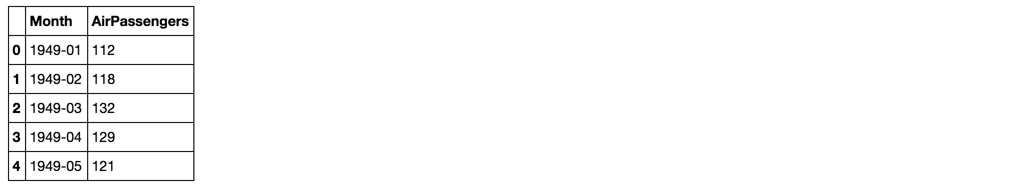
Our DataFrame clearly contains a Month and AirPassengers column. The Prophet library expects as input a DataFrame with one column containing the time information, and another column containing the metric that we wish to forecast. Importantly, the time column is expected to be of the datetime type, so let’s check the type of our columns:
df.dtypes
OutputMonth            object
AirPassengers     int64
dtype: object
Because the Month column is not of the datetime type, we’ll need to convert it:
df['Month'] = pd.DatetimeIndex(df['Month'])
df.dtypes
OutputMonth            datetime64[ns]
AirPassengers             int64
dtype: object
We now see that our Month column is of the correct datetime type.
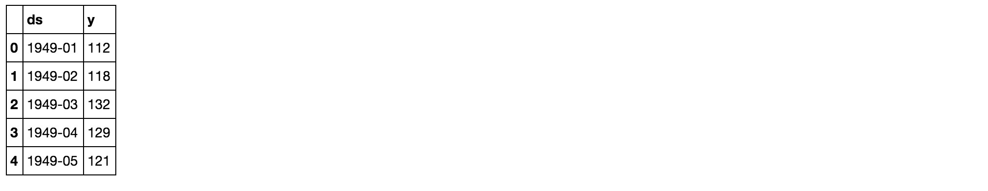
Prophet also imposes the strict condition that the input columns be named ds (the time column) and y (the metric column), so let’s rename the columns in our DataFrame:
df = df.rename(columns={'Month': 'ds',
                        'AirPassengers': 'y'})

df.head(5)
It is good practice to visualize the data we are going to be working with, so let’s plot our time series:
ax = df.set_index('ds').plot(figsize=(12, 8))
ax.set_ylabel('Monthly Number of Airline Passengers')
ax.set_xlabel('Date')

plt.show()
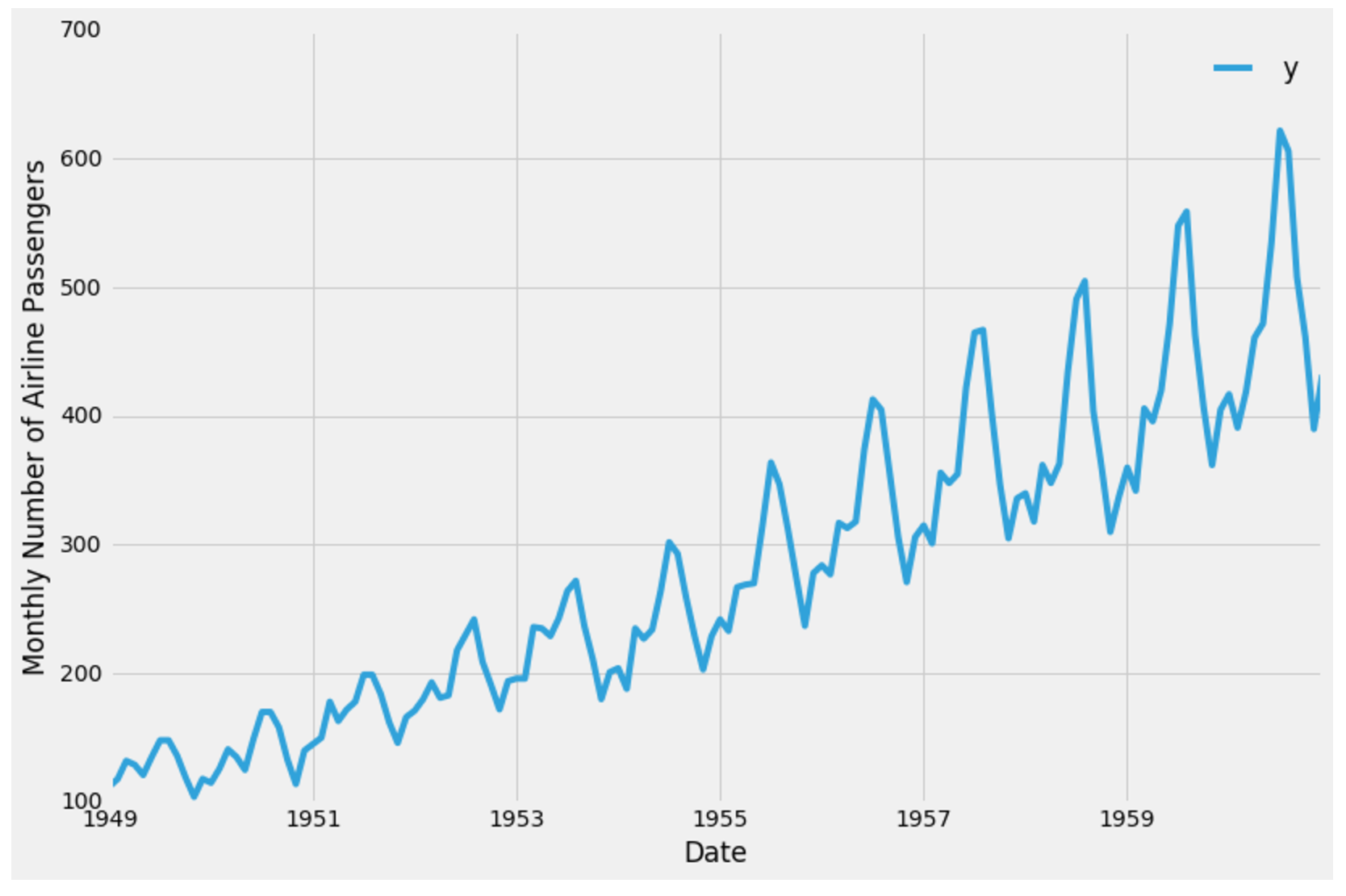
With our data now prepared, we are ready to use the Prophet library to produce forecasts of our time series.
Step 3 — Time Series Forecasting with Prophet
In this section, we will describe how to use the Prophet library to predict future values of our time series. The authors of Prophet have abstracted away many of the inherent complexities of time series forecasting and made it more intuitive for analysts and developers alike to work with time series data.
To begin, we must instantiate a new Prophet object. Prophet enables us to specify a number of arguments. For example, we can specify the desired range of our uncertainty interval by setting the interval_width parameter.
# set the uncertainty interval to 95% (the Prophet default is 80%)
my_model = Prophet(interval_width=0.95)
Now that our Prophet model has been initialized, we can call its fit method with our DataFrame as input. The model fitting should take no longer than a few seconds.
my_model.fit(df)
You should receive output similar to this:
Output<fbprophet.forecaster.Prophet at 0x110204080>
In order to obtain forecasts of our time series, we must provide Prophet with a new DataFrame containing a ds column that holds the dates for which we want predictions. Conveniently, we do not have to concern ourselves with manually creating this DataFrame, as Prophet provides the make_future_dataframe helper function:
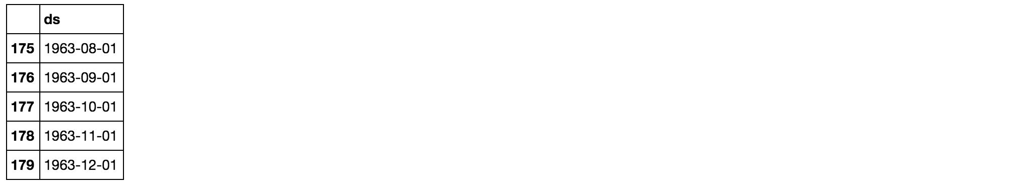
future_dates = my_model.make_future_dataframe(periods=36, freq='MS')
future_dates.tail()
In the code chunk above, we instructed Prophet to generate 36 datestamps in the future.
When working with Prophet, it is important to consider the frequency of our time series. Because we are working with monthly data, we clearly specified the desired frequency of the timestamps (in this case, MS is the start of the month). Therefore, the make_future_dataframe generated 36 monthly timestamps for us. In other words, we are looking to predict future values of our time series 3 years into the future.
The DataFrame of future dates is then used as input to the predict method of our fitted model.
forecast = my_model.predict(future_dates)
forecast[['ds', 'yhat', 'yhat_lower', 'yhat_upper']].tail()
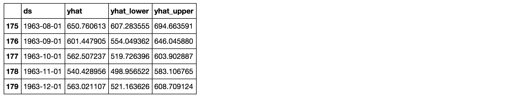
Prophet returns a large DataFrame with many interesting columns, but we subset our output to the columns most relevant to forecasting, which are:
ds: the datestamp of the forecasted valueyhat: the forecasted value of our metric (in Statistics,yhatis a notation traditionally used to represent the predicted values of a valuey)yhat_lower: the lower bound of our forecastsyhat_upper: the upper bound of our forecasts
A variation in values from the output presented above is to be expected as Prophet relies on Markov chain Monte Carlo (MCMC) methods to generate its forecasts. MCMC is a stochastic process, so values will be slightly different each time.
Prophet also provides a convenient function to quickly plot the results of our forecasts:
my_model.plot(forecast,
              uncertainty=True)
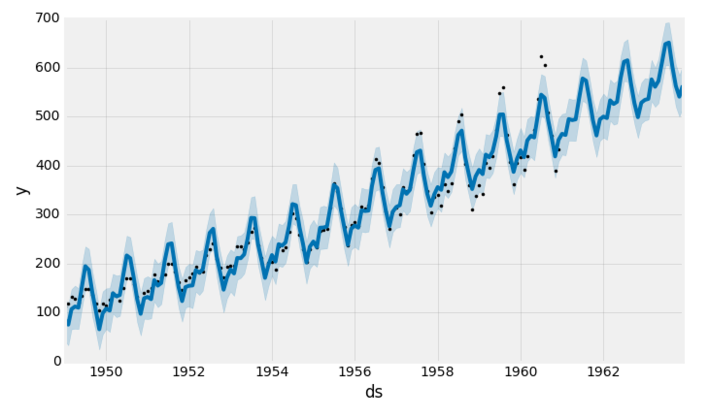
Prophet plots the observed values of our time series (the black dots), the forecasted values (blue line) and the uncertainty intervals of our forecasts (the blue shaded regions).
One other particularly strong feature of Prophet is its ability to return the components of our forecasts. This can help reveal how daily, weekly and yearly patterns of the time series contribute to the overall forecasted values:
my_model.plot_components(forecast)
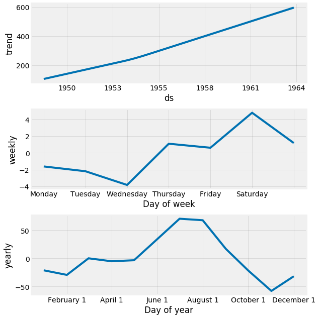
The plot above provides interesting insights. The first plot shows that the monthly volume of airline passengers has been linearly increasing over time. The second plot highlights the fact that the weekly count of passengers peaks towards the end of the week and on Saturday, while the third plot shows that the most traffic occurs during the holiday months of July and August.
Conclusion
In this tutorial, we described how to use the Prophet library to perform time series forecasting in Python. We have been using out-of-the box parameters, but Prophet enables us to specify many more arguments. In particular, Prophet provides the functionality to bring your own knowledge about time series to the table.
Here are a few additional things you could try:
- Assess the effect of holidays by including your prior knowledge on holiday months (for example, we know that the month of December is a holiday month). The official documentation on modeling holidays will be helpful.
- Change the range of your uncertainty intervals, or forecast further into the future.
For more practice, you could also try to load another time series dataset to produce your own forecasts. Overall, Prophet offers a number of compelling features, including the opportunity to tailor the forecasting model to the requirements of the user.
Thanks for learning with the DigitalOcean Community. Check out our offerings for compute, storage, networking, and managed databases.
Tutorial Series: Time Series Visualization and Forecasting
Time series are a pivotal component of data analysis. This series goes through how to handle time series visualization and forecasting in Python 3.
This textbox defaults to using Markdown to format your answer.
You can type !ref in this text area to quickly search our full set of tutorials, documentation & marketplace offerings and insert the link!


Get our biweekly newsletter
Sign up for Infrastructure as a Newsletter.

Hollie's Hub for Good
Working on improving health and education, reducing inequality, and spurring economic growth? We'd like to help.

Become a contributor
Get paid to write technical tutorials and select a tech-focused charity to receive a matching donation.

Check out AnticiPy which is an open-source tool for forecasting using Python and developed by Sky.
The goal of AnticiPy is to provide reliable forecasts for a variety of time series data, while requiring minimal user effort.
AnticiPy can handle trend as well as multiple seasonality components, such as weekly or yearly seasonality. There is built-in support for holiday calendars, and a framework for users to define their own event calendars. The tool is tolerant to data with gaps and null values, and there is an option to detect outliers and exclude them from the analysis.
Ease of use has been one of our design priorities. A user with no statistical background can generate a working forecast with a single line of code, using the default settings. The tool automatically selects the best fit from a list of candidate models, and detects seasonality components from the data. Advanced users can tune this list of models or even add custom model components, for scenarios that require it. There are also tools to automatically generate interactive plots of the forecasts (again, with a single line of code), which can be run on a Jupyter notebook, or exported as .html or .png files.
Check it out here: https://pypi.org/project/anticipy/
Do you know how uncertainty interval is calculated?
Thank you for creating such a great walkthrough. In your components visualisation, you’ve been able to display trend, weekly and yearly trends. However, in my notebook I only get the trend and yearly. Why is that?
Can we adapt this to train for weekly data??
INFO:fbprophet.forecaster:Disabling daily seasonality. Run prophet with daily_seasonality=True to override this. Initial log joint probability = -2.46502 Iter log prob ||dx|| ||grad|| alpha alpha0 # evals Notes 99 402.571 0.000207143 101.815 0.9661 0.9661 136
Iter log prob ||dx|| ||grad|| alpha alpha0 # evals Notes 199 402.966 1.93889e-06 74.3745 0.2165 0.7593 282
Iter log prob ||dx|| ||grad|| alpha alpha0 # evals Notes 217 402.968 8.45346e-06 60.1757 1.2e-07 0.001 339 LS failed, Hessian reset 247 402.968 1.74976e-08 64.7367 0.2863 0.2863 382
Optimization terminated normally: Convergence detected: relative gradient magnitude is below tolerance
this output is comming for me. Please help.
How are you getting a weekly trend when the data is at a monthly level? I would think that one can get monthly and yearly trend from a monthly data, but not weekly?
This comment has been deleted