By Adrien Payong and Shaoni Mukherjee

Before an AI product reaches large-scale adoption, its infrastructure must be designed to handle more than model accuracy. Inference systems in production require support for unpredictable traffic patterns, variable request sizes, strict latency constraints, and increasing compute costs. That’s why scaling machine learning inference is both a model engineering problem and a systems engineering challenge.
Machine learning services handling one million inference requests per day may sound impressive. While this averages only ~11.6 requests per second, traffic is rarely uniform—bursty patterns, uneven request rates, and variable prompt sizes are the norm. The first points of failure are usually not the model itself, but the serving system: unexpected queueing delays, GPU starvation, cost explosions, slow autoscaling, batching trade-offs, and gaps in observability. This article explores these failure modes, their causes, and strategies for detection and mitigation.
Key TakeAways
- The first failure at 1M inference requests/day is usually the serving system, not the model. Queueing, GPU contention, batching delays, autoscaling lag, and weak observability often break before model quality becomes an issue.
- Average RPS and average latency are misleading. Even though 1M requests/day averages about 11.6 RPS, real traffic is bursty, and p95/p99 latency reveals overload much earlier than average.
- High GPU utilization does not always mean high productivity. A GPU can look busy while useful throughput remains low because of memory pressure, KV-cache movement, poor batching, or pipeline stalls.
- Inference cost should be measured per token, not only per GPU hour. Long prompts, long outputs, retries, idle GPUs, and inefficient batching can make the cost grow faster than request volume.
- Production inference needs inference-specific observability and autoscaling signals. Teams should monitor queue depth, queue wait time, TTFT, p95/p99 latency, GPU memory, active sequences, tokens per second, retry rate, and cost per request.
Queueing Is Usually the First Bottleneck
Queueing is often the first symptom that the inference system is reaching its limits. Requests will start queueing up, waiting for GPU memory capacity, batching windows, or inference execution slots before the model itself begins to struggle. Queueing delays can be difficult to notice because they are typically hidden inside overall latency metrics. Queueing delays at 1M requests per day can easily lead to p95 and p99 latency problems, especially during peak traffic periods.
Why Average Latency Hides Overload
Queueing latency can fail silently before anything else. When incoming requests exceed processing capacity, they start queuing in a backlog. Some teams measure only average latency or requests per second(RPS), but those metrics obscure distribution. Some metrics must include time‑to‑first‑token (TTFT), end‑to‑end latency, and latency percentiles (p90, p95). This is because reporting averages hides tail latency experienced by users.
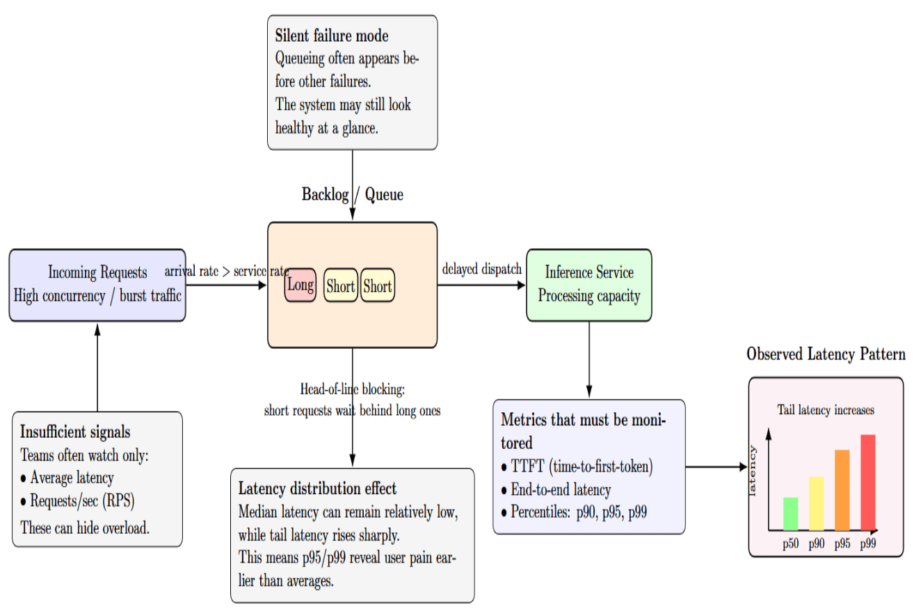
Tail latencies such as p95/p99 represent the worst‑case experience for a significant subset of users. High concurrency may cause shorter requests to be blocked by longer requests behind them (the head‑of‑line blocking problem). This can cause a high 95th percentile despite a low median.
Why p99 and p95 matter
Average latency can mask significant performance issues. The inference system may appear healthy on average, but a small percentage of users are experiencing long delays. p95 latency is the response time experienced by 95% of requests. p99 latency is the response time experienced by 99% of requests.
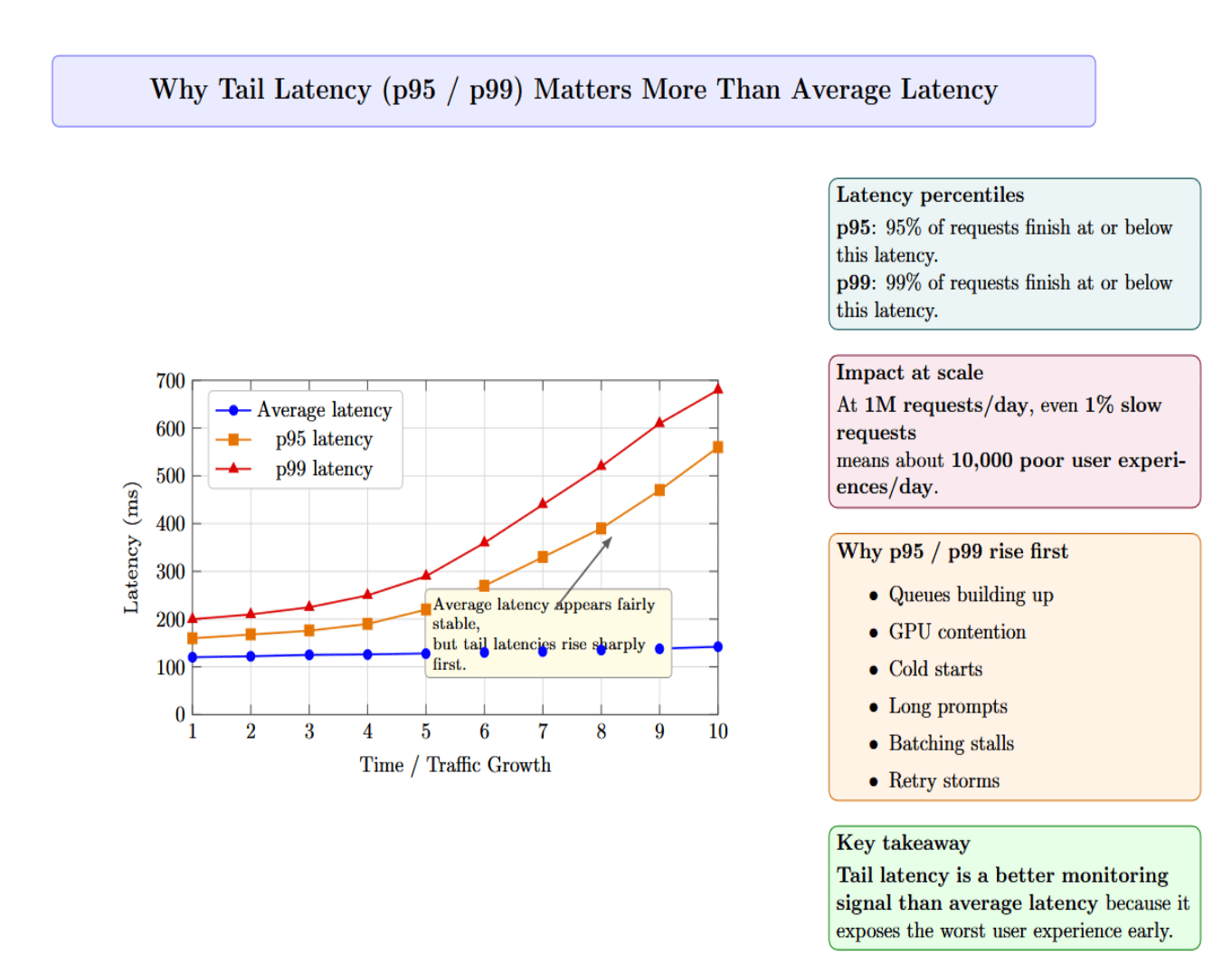
At 1M requests per day, even 1% of slow requests translates to roughly 10,000 poor user experiences daily. Typically, you’ll see p95 or p99 latency increasing first due to queues building up, GPU contention, cold starts, long prompts, batching stalls, or retry storms before average latency exposes the issue. For this reason, tail latency is a better metric for monitoring than average latency.
Why Average RPS Is Misleading
For example, consider a service that receives one million requests per day. If 40% of those requests hit during four hours of peak traffic, then you must serve approximately 28 requests per second during that peak period. This is more than twice the average request rate over the course of a day. If you don’t have enough capacity, queued requests will wait.
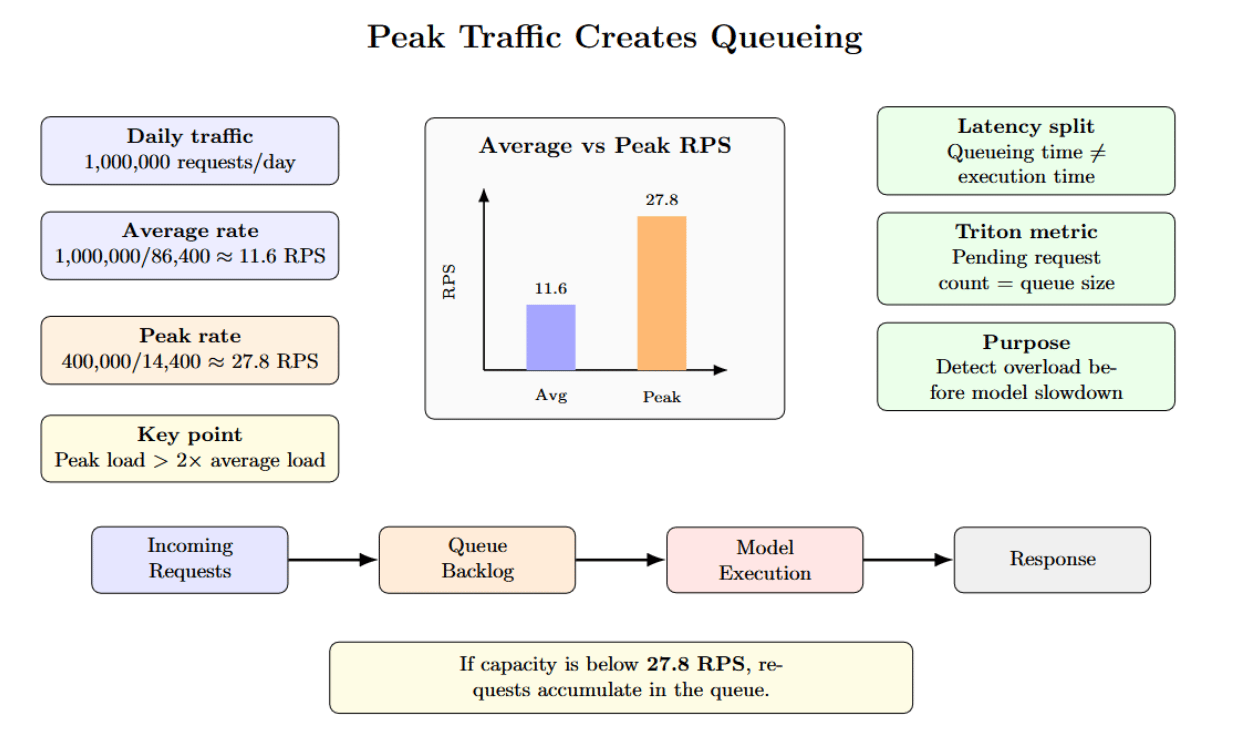
Queueing time is buried inside what is commonly referred to as “model latency”. Queueing time is actually isolated; Triton Inference Server’s metrics include pending request count (queue size) for each model. Queue length can be monitored separately from execution time to help determine when your bottleneck is occurring before the model.
GPU Contention Comes Next
After queuing, the next potential bottleneck is often GPU contention. High GPU utilization doesn’t always mean productivity. Memory pressure, KV cache churn, uneven batches, competing tenants, and at scale can all limit useful throughput even when utilization appears high.
GPU Utilization vs. Useful Throughput
The next most common failure mode after queuing is poor GPU utilization. Teams will notice that their GPU is busy, but still exhibits low throughput and high latency. Low utilization typically results from sub-optimal batching, inconsistent traffic, and pipeline stalls. GPUs often sit idle between requests because the traffic is bursty or the batches per request are small.
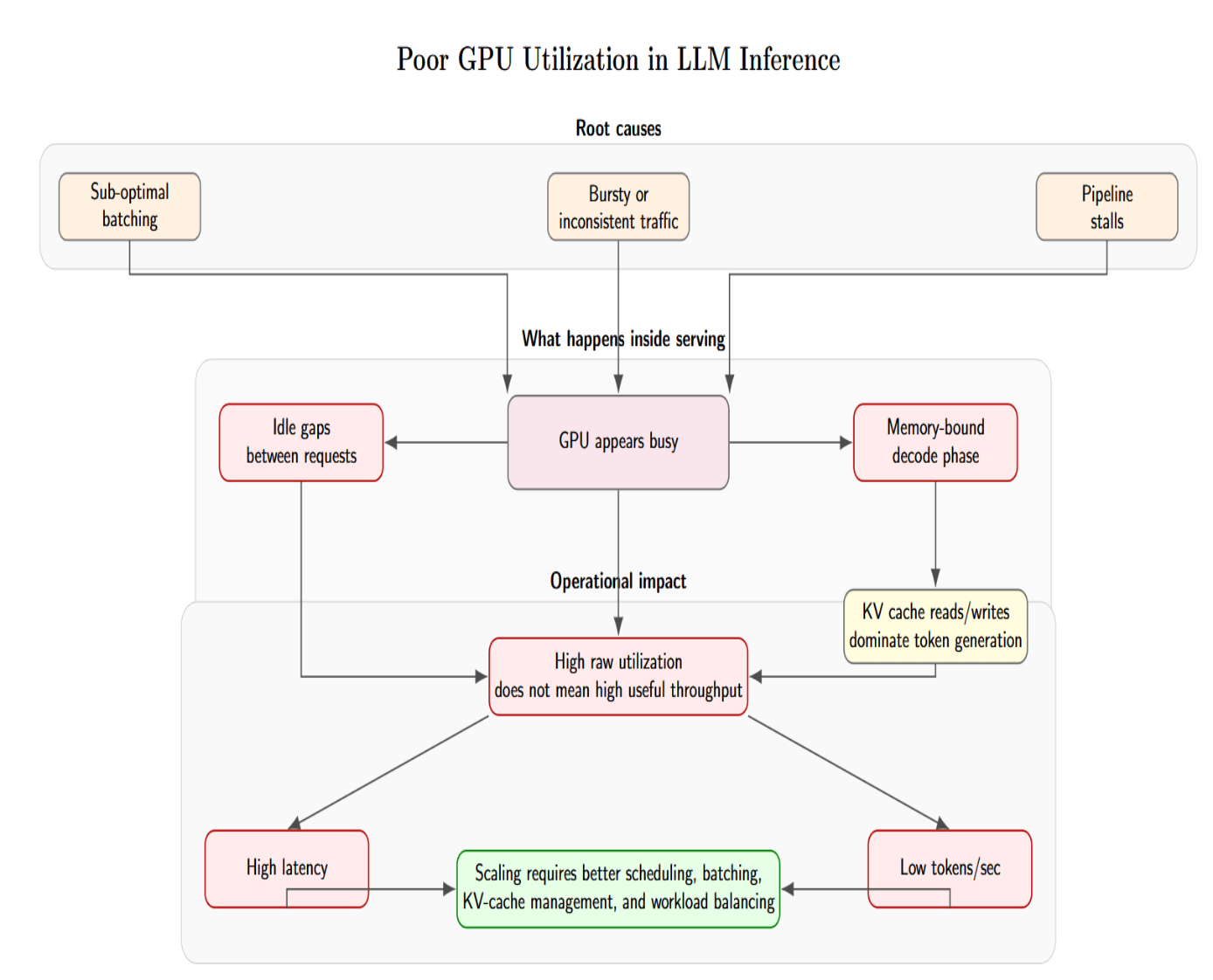
There’s also a more fundamental issue: the GPU may appear highly utilized, but the workload is memory-bound and not compute-bound. When serving LLMs, the decode phase constantly reads from and writes to the KV cache. If time is spent transferring tokens between the KV cache and GPU memory, the GPU can appear busy while failing to produce useful tokens per second.
This gap between raw utilization and productive throughput is why you can’t always throw more GPUs to increase capacity. Engineers must carefully tune batching, parallelism, request scheduling, memory usage, etc., and the surrounding serving architecture so the GPU remains continuously fed with useful work.
Multi‑Tenant Workloads and Batch Size Conflicts
When models or tenants share a GPU resource, they contend for GPU memory, compute, and the KV cache. Variation in sequence length produces stochastic queueing time. If one request reserves a large proportion of GPU memory, smaller requests may be unable to fit in memory. Requests with different batch sizes cause GPU underutilization. Triton supports multiple instances of the same model on each GPU through instance_group settings. It enables both high‑throughput and low‑throughput models to share the same GPU. Without careful scheduling, high‑throughput requests from one tenant can burst and consume resources, increasing latency to other tenants.
Cost Spikes Become Hard to Control
Cost is almost always the next failure mode after latency and GPU contention issues. Teams might incur infrastructure costs at a small scale, but at the production scale, inference costs depend on token volume, batching efficiency, model selection, and idle GPU time. This is why cost can rise faster than traffic when the serving system is not optimized.
Cost per Request vs. Cost per Token
The cost of inference doesn’t scale linearly with the number of requests. It’s a function of token volume, batching efficiency, retry behavior, and GPU idle time. Maybe you can serve more requests, but the determining factor for cost should be the total number of input and output tokens the platform is producing and how well the serving stack utilizes GPU capacity.
Rather than measuring inference economics by cost per GPU hour, NVIDIA reframes the problem as cost per token. You can calculate the cost per million tokens by dividing the cost per GPU hour by the number of tokens the GPU can process per second over one hour. The key factor is the denominator: tokens produced per second. It’s a measurement of how effectively the infrastructure turns GPU time into productive model output.
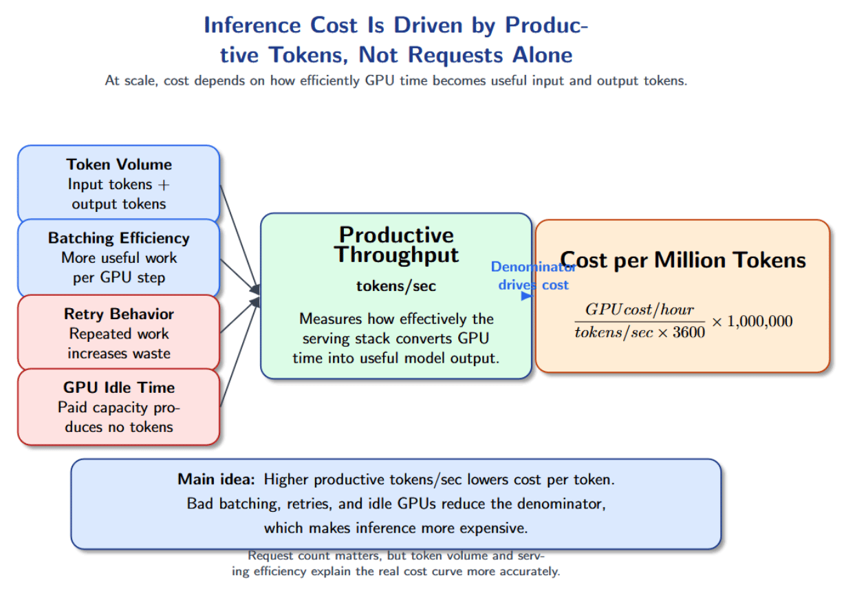
This also illustrates why looking at cost per GPU hour can be misleading. A cheaper GPU instance is not necessarily more economical if it produces fewer tokens per second or remains underutilized. You can think about the cost per request as follows:
cost per request = input token cost + output token cost + infrastructure overhead + retry overhead Long prompts mean more input token cost. Long outputs mean more output token cost. Retries duplicate work. Idle GPUs increase wasted infrastructure. During periods when batching is ineffective or traffic is bursty, the system pays for GPU time but does not turn that time into enough delivered tokens.
Why Retries and Idle GPUs Inflate Cost
Retries happen when requests time out or fail due to a queue backlog. Retries duplicate work and sends more tokens back through the pipeline. Idle GPUs add cost without producing tokens. Overprovisioning compute to meet peak traffic demands or using large models for small tasks increases cost. Engineers can react faster to cost spikes by right‑sizing models to tasks, applying quantization where quality allows, and tracking cost per request or per 1 k tokens in real time. Maximizing tokens per second reduces cost per token. You can reduce tokens per second with smart batching, scheduling models to stay as busy as possible, and maximizing your hardware.
Autoscaling Reacts Too Late
Autoscaling failures often occur after queues have formed. This tends to happen when scaling policies look only at CPU utilization. With GPU inference workloads, the CPU may look healthy while GPU memory is saturated, pending requests increase, and p99 latency is rising.
Better autoscaling signals for inference include queue depth, queue wait time, GPU memory utilization, active sequences, pending requests, TPS (tokens/sec), p95 latency, and time to first token. These signals reflect serving pressure more accurately than CPU utilization.
Cold starts are another factor making autoscaling painful. Starting up a new worker can take time to schedule the pod, attach a GPU, load model weights into GPU memory, warm up kernels, and join the load balancer. Autoscaling may add a new worker right as the users are experiencing latency.
For latency-sensitive inference, scale-to-zero is risky. A better approach is to keep a minimum number of warm workers, scale based on inference-specific metrics, and use predictive scaling when traffic patterns are known. The goal is to reduce overload duration, cold starts, and p99 latency during traffic spikes.
Batching Improves Throughput but Can Hurt Latency
Batching is the common method of improving inference throughput. The server groups incoming requests together so that each request goes straight to the GPU. The GPU can use batching to process multiple requests efficiently, leading to better hardware utilization and higher predictions/tokens per second.
However, batching creates a latency trade-off. The server may wait a short while so that it has enough requests for a better batch. While that may help throughput, it also increases queuing delay. Batching queue delay isn’t always bad. If you have offline workloads (think batch pipelines), then the extra queue delay usually isn’t a problem. However, if you have an interactive workload, batching can significantly degrade p95 and p99 latency.
The best batching strategy depends on the workload. Computer vision workloads and embedding mostly benefit from batching because their inputs are more predictable. Language models are harder to batch because prompts and outputs vary in length. A short request could be stuck waiting if it has to be batched with large requests.
Teams should tune batch size, preferred batch size, and maximum queue delay using realistic traffic patterns. The goal is to increase tokens per second or predictions per second without causing unacceptable tail latency.
Observability Breaks When Logs Are Not Enough
Logs might be sufficient to debug inference failures at a small scale. At 1M requests per day, that visualizes where latency is introduced.
Trace every request from API gateway → queue → model execution → token generation → post-processing → response. The production dashboard should separate application latency, queue latency, model execution time, time to first token, total generation time, error rate + retry rate, and cost. They become too noisy and incomplete. You need metrics, traces, dashboards, and runbooks.
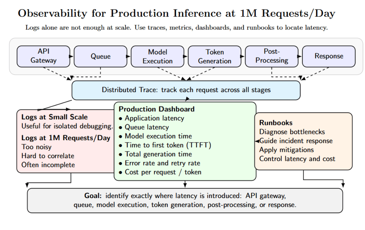
Teams running GPU inference should also track GPU utilization, GPU memory, number of active sequences, batch size, tokens per second, and cache hit/miss rate.
Debugging Real Inference Failures
The table below summarizes three common production inference incidents that appear when traffic increases or when workload patterns change. It connects each failure scenario to its likely causes and the practical checks engineers can use to diagnose and fix the problem quickly.
| Failure Scenario | Likely Causes | What to Check / How to Fix |
|---|---|---|
| Latency spikes with normal GPU utilization | Queue buildup; long prompts; poor batching; slow downstream services. | Check Triton pending request count; inspect batch size; increase worker replicas; tune max_queue_delay_microseconds; limit context length. |
| Cost spikes without traffic spikes | Longer outputs; retries from timeouts; inefficient batching; higher-tier models for all requests; KV-cache memory waste. | Track cost per request; monitor cost per 1K tokens; watch retry rate; reduce output length; limit generation steps; use smaller models where possible. |
| p99 latency explosion after launch | Bursty launch traffic; autoscaling lag; CPU-based scaling; GPU node provisioning delay; model loading delay. | Pre-provision warm capacity; scale on queue depth, GPU utilization, and p95 latency; test cold starts; use priority queues; apply rate limiting and backpressure. |
How to Prepare Before Reaching 1 M Requests/Day
Most of these inference failures can be avoided with some preparation. Teams should load-test their serving stack with expected prompt lengths, output lengths, and traffic, rather than generating synthetic fixed-length inputs. Try simulating real-world scenarios with tools like Triton Performance Analyzer or vLLM benchmarking to measure throughput, latency percentiles, and cost across different batch sizes, prompt sizes, and concurrency levels.
Production inference systems should classify requests into well-defined classes. Short, medium, long, streaming, batch, and high-priority requests should be sent to specific queues or serving pools. This way, lightweight classes won’t get blocked by long or slow requests. Rate limits and backpressure are important too — slow clients should never be allowed to consume capacity indefinitely.
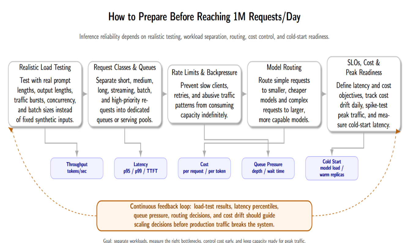
Model routing is another useful preparation step. You can configure a router to choose an appropriate model tier depending on the complexity of the request. Requests with simpler needs can be routed to cheaper, smaller models, while larger models can be used for more compute-intensive tasks. This helps manage costs without sacrificing quality.
Before scaling, teams should also define explicit latency and cost service level objectives. You should track cost per request daily and analyze any drift as soon as possible. Last, teams should spike traffic patterns expected at peak, and measure cold-start latency. If the latency budgets are strict, consider optimizing model load times or keeping warm replicas ready to serve traffic.
Practical Architecture for 1 M Requests/Day Inference
Below is a practical architecture for handling one million requests per day. It includes components for classification, queueing, routing, scheduling, observability, and cost control.
- API Gateway – Provides a single endpoint for clients. Performs authentication, rate limiting, and request validation. Enriches requests with metadata (userId, priority, etc.) and sends requests to the classifier.
- Request Classifier – Assigns incoming requests to a class based on prompt length and customer tier. This classification informs queueing and routing decisions.
- Priority Queue – Maintains separate queues for different classes. High‑priority queues have shorter maximum queue delay and are drained preferentially. Queue depth and wait time metrics trigger autoscaling.
- Model Router – Routes each request to the appropriate model/engine based on context. For example, it might send simple requests to a smaller model and route expensive requests to a larger model. Routing logic could also choose between vLLM, TensorRT‑LLM, or Triton backends.
- Inference Workers on GPU – Run the chosen model. Each worker performs continuous batching to serve many requests concurrently using dynamic scheduling to avoid head‑of‑line blocking. Workers publish metrics including tokens per second, number of active sequences, and GPU memory utilization.
- Monitoring and Cost Dashboard – Aggregate metrics from the API gateway, queue, router, and workers. It visualizes tail latencies, queue depth, tokens per sec, GPU utilization, and cost per request. Sends alerts when SLOs are violated or cost drifts are detected.
- Response Layer – Aggregates outputs, performs post‑processing (detokenization, streaming support), and sends responses back to the client. The response layer tracks metrics like time to first token and total generation time.
Key Metrics to Monitor
The following table summarises essential metrics for each category. Tracking these metrics provides visibility into bottlenecks, guides scaling decisions, and prevents silent cost drift.
| Category | Metric | Why It Matters |
|---|---|---|
| Traffic | Requests per second | Shows arrival rate and helps compare demand with per-instance throughput. |
| Latency | p50, p90, p95, p99 latency | Reveals tail latency and user-facing delays that averages can hide. |
| Queueing | Queue depth, nv_inference_pending_request_count, queue wait time |
Detects overload early and supports better autoscaling decisions. |
| GPU | GPU utilization, nv_gpu_utilization, GPU memory used |
Shows accelerator pressure and memory-related bottlenecks. |
| LLM Serving | Tokens per second, active sequences, time to first token | Measures generation performance and separates prefill from decode bottlenecks. |
| Batching | Average batch size, batch wait time, dynamic vs. continuous batching metrics | Shows batching efficiency and helps tune queue delay and batch parameters. |
| Reliability | Timeout rate, retry rate, error rate | Detects instability and failed request patterns. |
| Cost | Cost per request, cost per thousand tokens | Prevents silent cost drift from long outputs, retries, or idle GPUs. |
| Autoscaling | Pending pods, cold-start time, node provisioning time | Shows scaling delay and whether warm capacity is needed. |
Frequently Asked Questions
What is inference scaling?
Scaling inference is serving more prediction/generation requests while maintaining latency, throughput, reliability, and cost goals.
How many requests per second is 1M requests per day?
The average incoming traffic of 1 million requests per day equates to ~11.6 requests per second. However, most production systems still must plan for peak traffic and not average traffic.
Why does inference latency increase at scale?
Factors that can increase latency at scale include queueing, GPU saturation, batching delay, slow autoscaling, and long requests blocking short ones.
What causes GPU contention in inference workloads?
Contention can occur when multiple inference workloads compete for resources such as GPU memory, GPU compute, KV cache, model instance, and execution slot.
How do you reduce inference cost?
Run requests on the appropriate model tier; Improve batching, reduce retries, reduce idle GPU time, monitor token usage, and separate batch from latency-sensitive requests.
Conclusion
The thing that typically breaks first at 1M requests/day is not the model. It’s the control system around your model. Queueing latency, GPU contention, batching inefficiencies, autoscaling delays, and poor observability turn everyday traffic increases into firefighting.
large-scale inference teams approach serving as an engineering problem. They measure queue time and execution time separately. They tune GPU utilization without sacrificing p99 latency. They track their cost per request and proactively build fallback paths. Reliable inference at production scale doesn’t come from buying more compute. It comes from building a system that knows where, when, and why computing is being wasted.
Thanks for learning with the DigitalOcean Community. Check out our offerings for compute, storage, networking, and managed databases.
About the author(s)
I am a skilled AI consultant and technical writer with over four years of experience. I have a master’s degree in AI and have written innovative articles that provide developers and researchers with actionable insights. As a thought leader, I specialize in simplifying complex AI concepts through practical content, positioning myself as a trusted voice in the tech community.
With a strong background in data science and over six years of experience, I am passionate about creating in-depth content on technologies. Currently focused on AI, machine learning, and GPU computing, working on topics ranging from deep learning frameworks to optimizing GPU-based workloads.
Still looking for an answer?
This textbox defaults to using Markdown to format your answer.
You can type !ref in this text area to quickly search our full set of tutorials, documentation & marketplace offerings and insert the link!
 This work is licensed under a Creative Commons Attribution-NonCommercial- ShareAlike 4.0 International License.
Become a contributor for community
Get paid to write technical tutorials and select a tech-focused charity to receive a matching donation.

DigitalOcean Documentation
Full documentation for every DigitalOcean product.

Resources for startups and AI-native businesses
The Wave has everything you need to know about building a business, from raising funding to marketing your product.
The developer cloud
Scale up as you grow — whether you're running one virtual machine or ten thousand.

Start building today
From GPU-powered inference and Kubernetes to managed databases and storage, get everything you need to build, scale, and deploy intelligent applications.
