Technical Writer II

Introduction
If you are choosing between a star schema and a snowflake schema for a PostgreSQL analytics database, start with this rule: use a star schema when query speed and ETL simplicity are your primary constraints, and use a snowflake schema when storage efficiency, referential integrity, and frequently updated dimension attributes matter more.
Both schemas implement dimensional modeling for OLAP workloads. PostgreSQL supports both without extensions, and both run on DigitalOcean Managed PostgreSQL. If you are evaluating PostgreSQL against other database systems, the comparison of relational database management systems covers why PostgreSQL is commonly chosen for analytics use cases.
The difference between the two schemas is a trade-off between denormalization and normalization in the dimension tables that surround your central fact table. This tutorial walks through DDL examples for both patterns using a consistent retail sales scenario, compares EXPLAIN ANALYZE output for equivalent queries, and covers indexing and configuration for analytics workloads on managed PostgreSQL.
In this tutorial, you will learn how to implement star and snowflake schemas in PostgreSQL, evaluate their query performance using EXPLAIN ANALYZE, configure DigitalOcean Managed PostgreSQL for analytics workloads, and choose between the two patterns using a repeatable decision framework.
Key Takeaways
- A star schema denormalizes all dimension attributes into flat tables, producing fewer joins and faster aggregation queries at the cost of storage redundancy.
- A snowflake schema normalizes dimension hierarchies into additional lookup tables, reducing update anomalies and storage footprint but increasing join complexity.
- PostgreSQL uses hash joins for dimension lookups in both schemas;
work_memconfiguration directly affects performance when multi-join snowflake queries exceed available memory. - Star schema queries require fewer hash join operations than equivalent snowflake queries; the performance gap widens as fact table row counts increase and as
work_memdecreases relative to intermediate result set sizes. - BRIN indexes on sequential date columns reduce index size and maintenance overhead compared to B-tree indexes for large, append-only analytics fact tables where row values are correlated with insertion order.
- DigitalOcean Managed PostgreSQL allows configuring
work_memandmax_parallel_workers_per_gatherthrough the control panel, which affects multi-join query planning directly. - Use the decision framework near the end of this tutorial to match schema choice to fact table size, query patterns, and ETL maturity.
Prerequisites
Before following this tutorial, you need:
- A DigitalOcean Managed PostgreSQL cluster running PostgreSQL 15 or later (PostgreSQL 14 clusters remain supported if already provisioned).
psqlinstalled and connected to your cluster. See How To Install and Use PostgreSQL on Ubuntu 22.04 for connection instructions.- A database named
analyticscreated on the cluster:CREATE DATABASE analytics; - Basic familiarity with SQL
SELECT,JOIN, andGROUP BYsyntax.
What Is a Star Schema in PostgreSQL
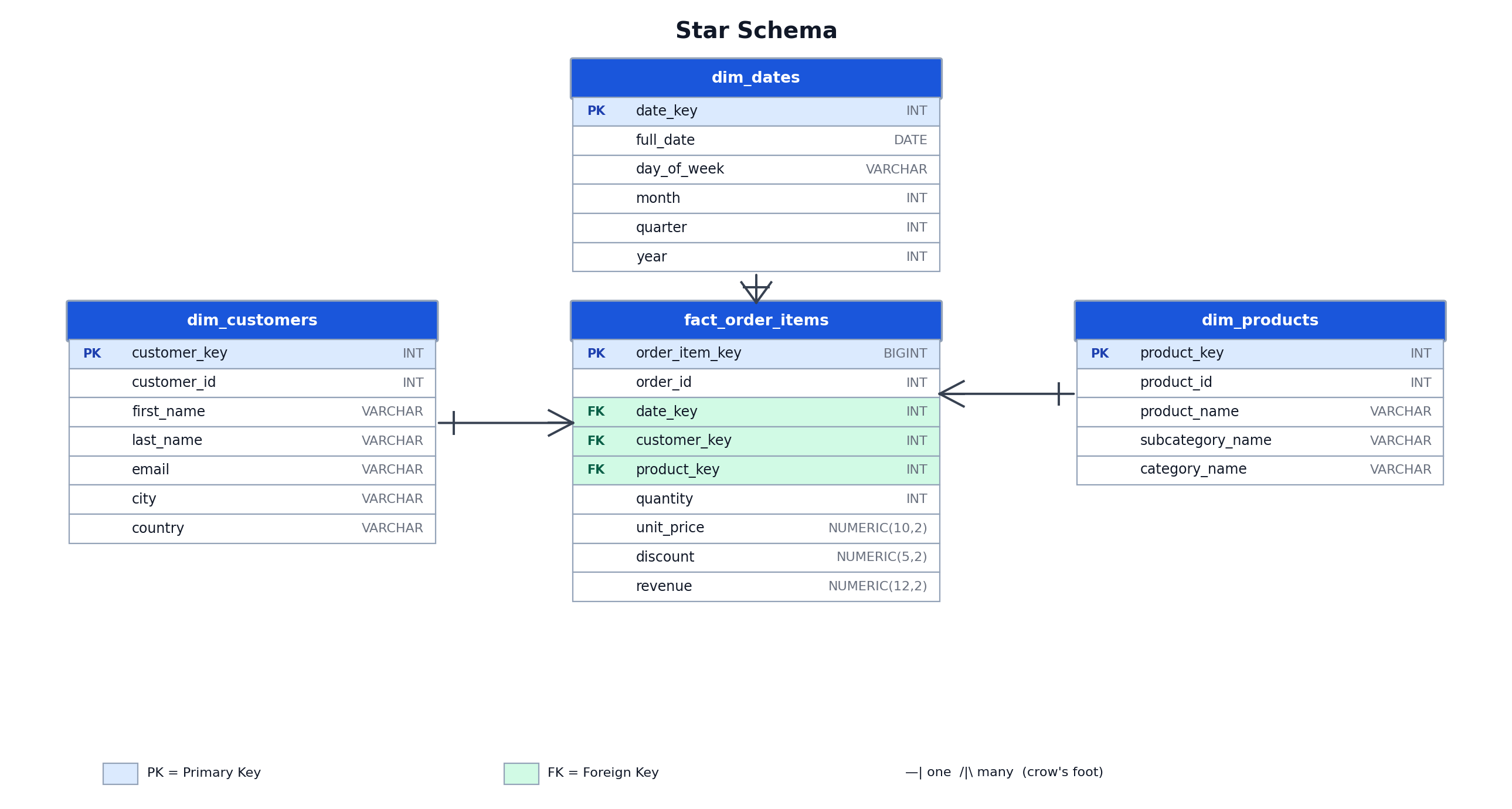
A star schema organizes analytics data into a central fact table surrounded by flat dimension tables. The shape, and the name, comes from the ER diagram: one table at the center with all dimension tables pointing outward.
Core Components: Fact Tables and Flat Dimension Tables
A star schema consists of a central fact table surrounded by flat dimension tables. The fact table stores measurable events: order line items, page views, or sensor readings. Dimension tables store the descriptive context for those events: product attributes, customer details, and date hierarchies.
In a star schema, dimension tables are denormalized. All attributes for a concept, such as a product, are stored in a single table, including both subcategory_name and category_name. A query aggregating revenue by product category joins the fact table to a single dimension table. The name “star schema” describes the visual shape of the entity-relationship diagram, with the fact table at the center and dimension tables radiating outward.
Star Schema DDL Example (Retail Sales Scenario)
CREATE TABLE dim_dates (
    date_key      INTEGER PRIMARY KEY,
    full_date     DATE        NOT NULL,
    day_of_week   VARCHAR(10) NOT NULL,
    month         INTEGER     NOT NULL,
    quarter       INTEGER     NOT NULL,
    year          INTEGER     NOT NULL
);

CREATE TABLE dim_customers (
    customer_key  INTEGER GENERATED BY DEFAULT AS IDENTITY PRIMARY KEY,
    customer_id   INTEGER      NOT NULL UNIQUE,
    first_name    VARCHAR(100) NOT NULL,
    last_name     VARCHAR(100) NOT NULL,
    email         VARCHAR(255) NOT NULL,
    city          VARCHAR(100),
    country       VARCHAR(100)
);

CREATE TABLE dim_products (
    product_key       INTEGER GENERATED BY DEFAULT AS IDENTITY PRIMARY KEY,
    product_id        INTEGER      NOT NULL UNIQUE,
    product_name      VARCHAR(255) NOT NULL,
    subcategory_name  VARCHAR(100) NOT NULL,
    category_name     VARCHAR(100) NOT NULL
);

CREATE TABLE fact_order_items (
    order_item_key  BIGINT GENERATED BY DEFAULT AS IDENTITY PRIMARY KEY,
    order_id        INTEGER       NOT NULL,
    date_key        INTEGER       NOT NULL REFERENCES dim_dates(date_key),
    customer_key    INTEGER       NOT NULL REFERENCES dim_customers(customer_key),
    product_key     INTEGER       NOT NULL REFERENCES dim_products(product_key),
    quantity        INTEGER       NOT NULL,
    unit_price      NUMERIC(10,2) NOT NULL,
    discount        NUMERIC(5,2)  NOT NULL DEFAULT 0,
    revenue         NUMERIC(12,2) NOT NULL
);
The dim_products table stores subcategory_name and category_name as direct columns. If a category name changes, every matching row in dim_products must be updated individually.
When the Star Schema Is the Right Choice
The star schema is the right default for most analytics workloads. If your BI tool runs aggregation queries against a single dimension at a time, the flat structure means analysts can write straightforward two-join queries without navigating a hierarchy. Tools that generate SQL automatically, such as Metabase or Looker, tend to produce cleaner plans against star schemas than against normalized ones.
The other condition that favors a star schema is ETL pipeline maturity. Denormalizing before load requires a tested, reliable pipeline. If yours is stable and dimension attributes in your source system change rarely, you will not miss the update convenience that snowflake schemas provide. Start with a star schema when simplicity matters more than storage.
What Is a Snowflake Schema in PostgreSQL
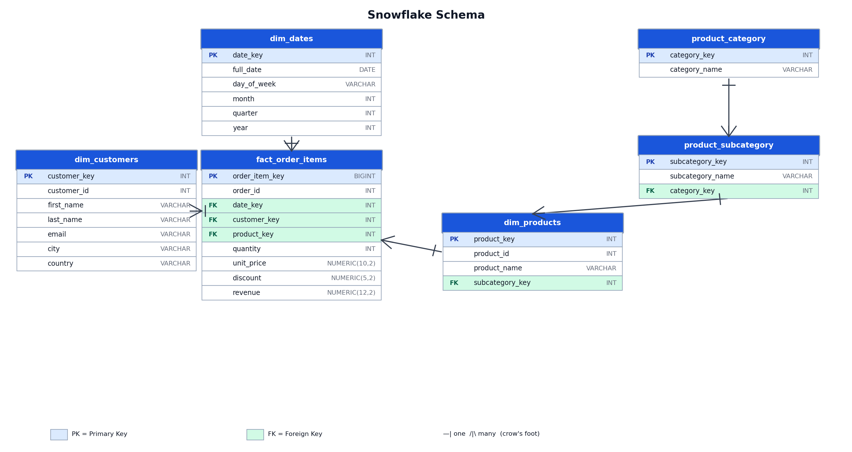
A snowflake schema starts with the same fact table but normalizes the dimension tables into additional lookup layers. The result is fewer redundant strings stored in the database and more joins required per query.
How Normalization Extends the Dimension Tables
A snowflake schema applies normalization to dimension tables. Instead of storing category_name directly in dim_products, the product dimension references a product_subcategory table, which in turn references a product_category table. This removes the functional dependency between subcategory_name and category_name from dim_products.
The trade-off is that queries requiring category-level aggregation must now join three tables instead of one, traversing the hierarchy from fact_order_items through dim_products, product_subcategory, and product_category.
Snowflake Schema DDL Example (Same Retail Sales Scenario)
CREATE TABLE product_category (
    category_key   INTEGER GENERATED BY DEFAULT AS IDENTITY PRIMARY KEY,
    category_name  VARCHAR(100) NOT NULL
);

CREATE TABLE product_subcategory (
    subcategory_key   INTEGER GENERATED BY DEFAULT AS IDENTITY PRIMARY KEY,
    subcategory_name  VARCHAR(100) NOT NULL,
    category_key      INTEGER      NOT NULL REFERENCES product_category(category_key)
);

CREATE TABLE dim_dates (
    date_key      INTEGER PRIMARY KEY,
    full_date     DATE        NOT NULL,
    day_of_week   VARCHAR(10) NOT NULL,
    month         INTEGER     NOT NULL,
    quarter       INTEGER     NOT NULL,
    year          INTEGER     NOT NULL
);

CREATE TABLE dim_customers (
    customer_key  INTEGER GENERATED BY DEFAULT AS IDENTITY PRIMARY KEY,
    customer_id   INTEGER      NOT NULL UNIQUE,
    first_name    VARCHAR(100) NOT NULL,
    last_name     VARCHAR(100) NOT NULL,
    email         VARCHAR(255) NOT NULL,
    city          VARCHAR(100),
    country       VARCHAR(100)
);

CREATE TABLE dim_products (
    product_key      INTEGER GENERATED BY DEFAULT AS IDENTITY PRIMARY KEY,
    product_id       INTEGER      NOT NULL UNIQUE,
    product_name     VARCHAR(255) NOT NULL,
    subcategory_key  INTEGER      NOT NULL REFERENCES product_subcategory(subcategory_key)
);

CREATE TABLE fact_order_items (
    order_item_key  BIGINT GENERATED BY DEFAULT AS IDENTITY PRIMARY KEY,
    order_id        INTEGER       NOT NULL,
    date_key        INTEGER       NOT NULL REFERENCES dim_dates(date_key),
    customer_key    INTEGER       NOT NULL REFERENCES dim_customers(customer_key),
    product_key     INTEGER       NOT NULL REFERENCES dim_products(product_key),
    quantity        INTEGER       NOT NULL,
    unit_price      NUMERIC(10,2) NOT NULL,
    discount        NUMERIC(5,2)  NOT NULL DEFAULT 0,
    revenue         NUMERIC(12,2) NOT NULL
);
When the Snowflake Schema Is the Right Choice
The snowflake schema earns its complexity when dimension attributes change frequently. If your product catalog is reorganized quarterly, updating one row in product_category is considerably cheaper than running a batch UPDATE across 20,000 rows in dim_products. At scale, that difference in update cost is not theoretical.
Two other cases favor snowflake: shared dimensions and data governance requirements. If a product_category table is referenced by both a sales fact table and an inventory fact table, normalizing it once prevents the two fact tables from diverging on category names. For environments where referential integrity must be enforced at the database level rather than in the application layer, the foreign key chain in a snowflake schema does that work automatically.
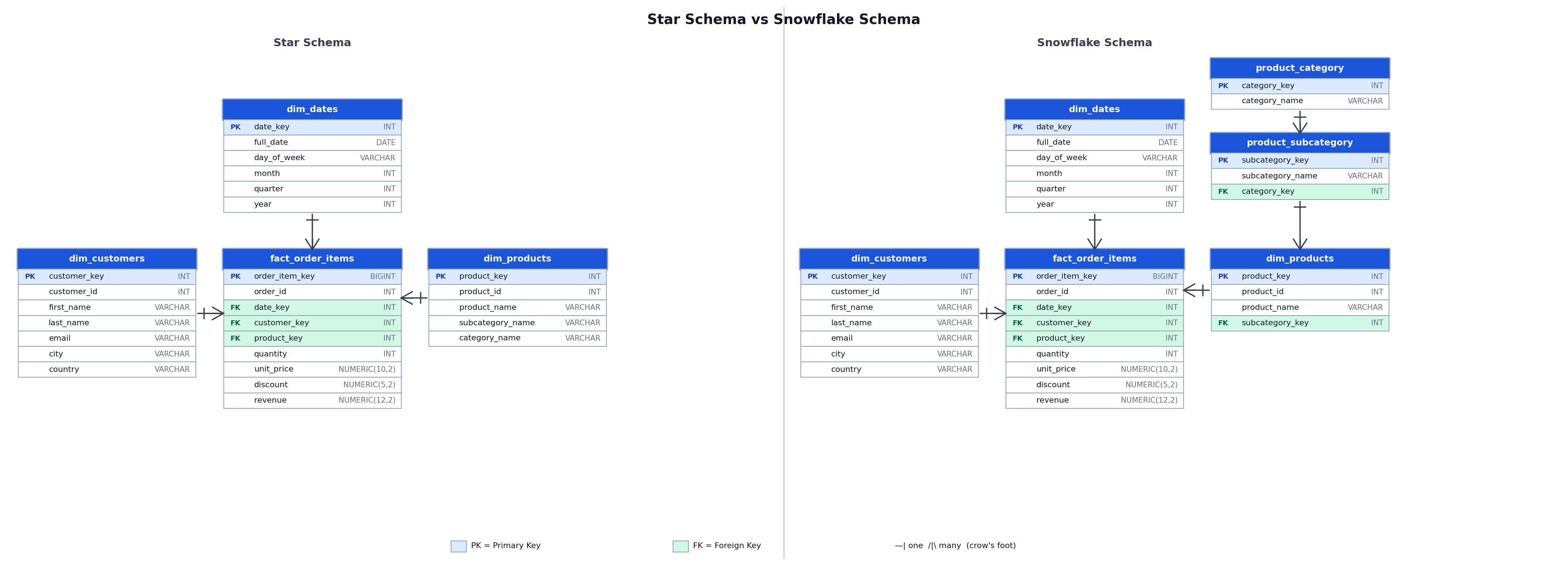
Star Schema vs Snowflake Schema: Direct Comparison
The practical difference between the two schemas is where you pay the cost: at query time with snowflake, or at ETL load time with star. The subsections below quantify that trade-off across the dimensions that matter most in production.
Query Complexity and Join Count
A star schema query joining fact_order_items to dim_products and dim_dates requires two joins to produce revenue by category and quarter. The equivalent snowflake query requires four joins: fact_order_items to dim_products, dim_products to product_subcategory, product_subcategory to product_category, and fact_order_items to dim_dates.
PostgreSQL handles additional hash joins efficiently when the smaller dimension tables fit in memory. However, each additional join increases planning time and the risk of a suboptimal join order at high row counts.
Storage Footprint and Data Redundancy
The storage math is straightforward. Take dim_products at 20,000 rows: storing category_name and subcategory_name as VARCHAR(100) columns on every row costs roughly 4 MB for those attributes alone. Move them into product_category (5 rows) and product_subcategory (2,800 rows), and the same information fits in under 50 KB. That is a 98% reduction for two columns.
In practice, this rarely drives the schema decision at the dimension table level. The fact table holds integer foreign keys in both schemas, so the real storage cost difference is in the dimension tables, not in fact_order_items. Where the savings become meaningful is when dimension tables have hundreds of thousands of rows with multiple low-cardinality VARCHAR attributes, which is common in product and geography hierarchies.
ETL Pipeline and Data Loading Complexity
Loading a star schema means your ETL pipeline owns the denormalization step. Before inserting into dim_products, the pipeline has to join the source product table with category and subcategory lookups and flatten the result into a single row. When that pipeline is well-tested, this is a one-time cost. When it is not, you will see category mismatches propagate silently into the dimension table.
A snowflake schema shifts that burden. The normalized structure maps more closely to how source systems store data, so dimension loads require fewer transformations. The trade-off is that incremental loads need to maintain consistency across product_category, product_subcategory, and dim_products in the correct order. Foreign key constraints will catch violations, but the coordination overhead is real.
Maintenance and Update Anomalies
A star schema is susceptible to update anomalies. If a product category name changes, every row in dim_products carrying that category_name must be updated. With slowly changing dimension (SCD) Type 1 patterns, this can require batch updates across large dimension tables.
A snowflake schema eliminates this for normalized attributes. Updating category_name in product_category propagates implicitly to all products in that category through the foreign key relationship, at the cost of one row update.
Comparison Table
| Schema | Query Speed | Storage Efficiency | Join Complexity | ETL Complexity | Best Fit Use Case |
|---|---|---|---|---|---|
| Star schema | Faster for most aggregations; fewer joins | Lower; redundant attribute strings in dimension rows | Low; 1-2 joins for typical analytical queries | Higher; pipeline must denormalize before load | BI reporting, dashboard queries, stable dimensions |
| Snowflake schema | Slower at scale; 2+ additional joins per hierarchy level | Higher; normalized attributes stored once | Higher; 3-5 joins for hierarchy-traversing queries | Lower; pipeline mirrors source structure more closely | Data governance environments, frequently updated dimensions, shared lookup tables |
Generating Test Data for Reproducible Benchmarks
The EXPLAIN ANALYZE outputs in the next section were collected on a production-representative dataset with a larger date range than the generator below. Run these generate_series scripts against your analytics database to populate a functionally equivalent dataset for schema validation and comparative benchmarking. Your plan row counts and timings will differ proportionally; the relative difference between star and snowflake query performance is consistent across dataset sizes at this scale.
Populate dim_dates with one row per calendar day from 2020 through 2025 (2,192 rows):
INSERT INTO dim_dates (date_key, full_date, day_of_week, month, quarter, year)
SELECT
    TO_CHAR(d, 'YYYYMMDD')::INTEGER,
    d::DATE,
    TO_CHAR(d, 'FMDay'),
    EXTRACT(MONTH FROM d)::INTEGER,
    EXTRACT(QUARTER FROM d)::INTEGER,
    EXTRACT(YEAR FROM d)::INTEGER
FROM generate_series('2020-01-01'::DATE, '2025-12-31'::DATE, '1 day') d;
Populate dim_customers with 50,000 rows:
INSERT INTO dim_customers (customer_id, first_name, last_name, email, city, country)
SELECT
    i,
    'First' || i,
    'Last' || i,
    'customer' || i || '@example.com',
    (ARRAY['New York','San Francisco','Chicago','Austin','Seattle'])[1 + (i % 5)],
    'US'
FROM generate_series(1, 50000) i;
Populate dim_products with 20,000 rows (star schema version):
INSERT INTO dim_products (product_id, product_name, subcategory_name, category_name)
SELECT
    i,
    'Product ' || i,
    (ARRAY['Laptops','Tablets','Phones','Monitors','Accessories',
           'Chairs','Desks','Shelves','Lamps','Rugs',
           'Jackets','Shirts','Pants','Shoes','Hats',
           'Bats','Balls','Nets','Gloves','Helmets',
           'Pans','Knives','Bowls','Plates','Cups'])[1 + (i % 25)],
    (ARRAY['Electronics','Furniture','Clothing','Sports','Kitchen'])[1 + (i % 5)]
FROM generate_series(1, 20000) i;
Populate fact_order_items with approximately 2.7 million rows:
INSERT INTO fact_order_items (order_id, date_key, product_key, customer_key, quantity, unit_price, discount, revenue)
SELECT
    (random() * 500000 + 1)::INTEGER,
    TO_CHAR('2020-01-01'::DATE + floor(random() * 2192)::INTEGER, 'YYYYMMDD')::INTEGER,
    (random() * 19999 + 1)::INTEGER,
    (random() * 49999 + 1)::INTEGER,
    v.quantity,
    v.unit_price,
    v.discount,
    ROUND((v.quantity * v.unit_price) * (1 - v.discount), 2) AS revenue
FROM generate_series(1, 2700000)
CROSS JOIN LATERAL (
    SELECT
        (random() * 10 + 1)::INTEGER         AS quantity,
        (random() * 500 + 10)::NUMERIC(10,2) AS unit_price,
        0::NUMERIC(5,2)                     AS discount
) v;
Run ANALYZE after loading to update planner statistics before benchmarking:
psql -d analytics -c "ANALYZE dim_dates, dim_customers, dim_products, fact_order_items;"
The star and snowflake versions of dim_products have incompatible column definitions, and fact_order_items references whichever version exists. Benchmark the two schemas in separate databases, or drop and recreate fact_order_items and dim_products with the snowflake DDL before running the block below. Running both schema definitions in the same database without recreating these tables will fail because the snowflake INSERT omits the subcategory_name and category_name columns that the star dim_products requires.
For the snowflake schema benchmark, populate the normalized dimension tables using the same 5-category, 2,800-subcategory structure (560 subcategories per category):
INSERT INTO product_category (category_name)
VALUES ('Electronics'), ('Furniture'), ('Clothing'), ('Sports'), ('Kitchen');

INSERT INTO product_subcategory (subcategory_name, category_key)
SELECT
    pc.category_name || ' Sub ' || s,
    pc.category_key
FROM product_category pc
CROSS JOIN generate_series(1, 560) s;

INSERT INTO dim_products (product_id, product_name, subcategory_key)
SELECT
    i,
    'Product ' || i,
    (SELECT subcategory_key
     FROM product_subcategory
     ORDER BY subcategory_key
     OFFSET (i % 2800) LIMIT 1)
Run ANALYZE on the snowflake dimension tables after loading:
psql -d analytics -c "ANALYZE product_category, product_subcategory;"
Query Performance on PostgreSQL: What the Numbers Show
Schema choice affects query plans in two measurable ways: join count and hash table memory usage. The EXPLAIN ANALYZE outputs below show both on the same 2.7 million-row fact table so the cost difference is directly comparable.
EXPLAIN ANALYZE Output for a Star Schema Aggregation Query
The EXPLAIN ANALYZE outputs below were generated on a DigitalOcean Managed PostgreSQL 15 cluster (4 vCPU, 8 GB RAM) with work_mem set to 64 MB. Row counts and timing values will differ on your cluster based on table statistics, memory configuration, and PostgreSQL version. The relative difference between the two schema types is representative of a denormalized vs. normalized dimension hierarchy at this row count.
This query aggregates revenue by product category and quarter on a fact_order_items table with approximately 2.7 million rows.
EXPLAIN ANALYZE
SELECT
    dp.category_name,
    dd.year,
    dd.quarter,
    SUM(foi.revenue)             AS total_revenue,
    COUNT(DISTINCT foi.order_id) AS order_count
FROM fact_order_items foi
JOIN dim_products dp ON foi.product_key = dp.product_key
JOIN dim_dates    dd ON foi.date_key    = dd.date_key
WHERE dd.year = 2023
  AND dp.category_name = 'Electronics'
GROUP BY dp.category_name, dd.year, dd.quarter
ORDER BY dd.quarter;
HashAggregate  (cost=84321.50..84325.80 rows=16 width=48)
               (actual time=412.344..412.591 rows=4 loops=1)
  Group Key: dp.category_name, dd.year, dd.quarter
  ->  Hash Join  (cost=1628.90..82944.30 rows=89918 width=32)
                 (actual time=20.344..387.801 rows=89918 loops=1)
        Hash Cond: (foi.date_key = dd.date_key)
        ->  Hash Join  (cost=1592.00..71308.20 rows=540000 width=28)
                       (actual time=18.211..298.112 rows=540000 loops=1)
              Hash Cond: (foi.product_key = dp.product_key)
              ->  Seq Scan on fact_order_items foi
                    (cost=0.00..52130.00 rows=2700000 width=24)
                    (actual time=0.021..142.430 rows=2700000 loops=1)
              ->  Hash  (cost=1592.00..1592.00 rows=4000 width=20)
                    (actual time=10.411..10.412 rows=4000 loops=1)
                    Buckets: 4096  Batches: 1  Memory Usage: 309kB
                    ->  Seq Scan on dim_products dp
                          (cost=0.00..1592.00 rows=4000 width=20)
                          (actual time=0.011..6.322 rows=4000 loops=1)
                          Filter: (category_name = 'Electronics')
                          Rows Removed by Filter: 16000
        ->  Hash  (cost=36.90..36.90 rows=365 width=12)
                  (actual time=2.511..2.512 rows=365 loops=1)
              Buckets: 1024  Batches: 1  Memory Usage: 26kB
              ->  Seq Scan on dim_dates dd
                    (cost=0.00..36.90 rows=365 width=12)
                    (actual time=0.009..1.234 rows=365 loops=1)
                    Filter: (year = 2023)
                    Rows Removed by Filter: 1827
Planning Time: 2.341 ms
Execution Time: 413.019 ms
PostgreSQL chose hash joins for both dimension lookups. The filter on category_name runs against the in-memory hash of dim_products, so all 2.7 million fact rows are read exactly once.
EXPLAIN ANALYZE Output for the Equivalent Snowflake Schema Query
EXPLAIN ANALYZE
SELECT
    pc.category_name,
    dd.year,
    dd.quarter,
    SUM(foi.revenue)             AS total_revenue,
    COUNT(DISTINCT foi.order_id) AS order_count
FROM fact_order_items  foi
JOIN dim_products        dp ON foi.product_key    = dp.product_key
JOIN product_subcategory ps ON dp.subcategory_key = ps.subcategory_key
JOIN product_category    pc ON ps.category_key    = pc.category_key
JOIN dim_dates           dd ON foi.date_key        = dd.date_key
WHERE dd.year = 2023
  AND pc.category_name = 'Electronics'
GROUP BY pc.category_name, dd.year, dd.quarter
ORDER BY dd.quarter;
HashAggregate  (cost=99812.40..99816.70 rows=16 width=48)
               (actual time=498.712..498.981 rows=4 loops=1)
  Group Key: pc.category_name, dd.year, dd.quarter
  ->  Hash Join  (cost=505.95..98180.20 rows=89918 width=32)
                 (actual time=22.341..471.229 rows=89918 loops=1)
        Hash Cond: (foi.date_key = dd.date_key)
        ->  Hash Join  (cost=469.05..95100.40 rows=540000 width=28)
                       (actual time=20.114..421.902 rows=540000 loops=1)
              Hash Cond: (ps.category_key = pc.category_key)
              ->  Hash Join  (cost=468.00..88444.30 rows=2700000 width=32)
                             (actual time=12.123..360.112 rows=2700000 loops=1)
                    Hash Cond: (dp.subcategory_key = ps.subcategory_key)
                    ->  Hash Join  (cost=412.00..80305.60 rows=2700000 width=28)
                                   (actual time=8.344..288.112 rows=2700000 loops=1)
                          Hash Cond: (foi.product_key = dp.product_key)
                          ->  Seq Scan on fact_order_items foi
                                (cost=0.00..52130.00 rows=2700000 width=24)
                                (actual time=0.021..142.430 rows=2700000 loops=1)
                          ->  Hash  (cost=412.00..412.00 rows=20000 width=8)
                                (actual time=8.111..8.112 rows=20000 loops=1)
                                Buckets: 32768  Batches: 1  Memory Usage: 940kB
                                ->  Seq Scan on dim_products dp
                                      (cost=0.00..412.00 rows=20000 width=8)
                                      (actual time=0.011..3.902 rows=20000 loops=1)
                    ->  Hash  (cost=56.00..56.00 rows=2800 width=8)
                          (actual time=3.211..3.212 rows=2800 loops=1)
                          Buckets: 4096  Batches: 1  Memory Usage: 142kB
                          ->  Seq Scan on product_subcategory ps
                                (cost=0.00..56.00 rows=2800 width=8)
                                (actual time=0.009..1.512 rows=2800 loops=1)
              ->  Hash  (cost=1.05..1.05 rows=1 width=12)
                        (actual time=0.018..0.019 rows=1 loops=1)
                    Buckets: 1024  Batches: 1  Memory Usage: 9kB
                    ->  Seq Scan on product_category pc
                          (cost=0.00..1.05 rows=1 width=12)
                          (actual time=0.007..0.011 rows=1 loops=1)
                          Filter: (category_name = 'Electronics')
                          Rows Removed by Filter: 4
        ->  Hash  (cost=36.90..36.90 rows=365 width=12)
                  (actual time=2.511..2.512 rows=365 loops=1)
              Buckets: 1024  Batches: 1  Memory Usage: 26kB
              ->  Seq Scan on dim_dates dd
                    (cost=0.00..36.90 rows=365 width=12)
                    (actual time=0.009..1.234 rows=365 loops=1)
                    Filter: (year = 2023)
                    Rows Removed by Filter: 1827
Planning Time: 3.812 ms
Execution Time: 499.621 ms
The snowflake query ran in 499 ms against 413 ms for the star schema query, a 21% difference on the same 2.7 million fact rows. In the plan shown, PostgreSQL joins dim_products to the full product_subcategory set (2,800 rows) before applying the pc.category_name = 'Electronics' filter at the product_category join. Depending on table statistics and configuration, the planner may instead choose a join order that applies the category restriction earlier.
Index Strategies for Fact Tables on Managed PostgreSQL
Three index strategies address the most common analytics bottlenecks on fact_order_items.
BRIN (Block Range Index) is efficient for columns where values are correlated with physical storage order, which is typical for append-only fact tables loaded in date order:
CREATE INDEX idx_fact_order_items_date_brin
    ON fact_order_items USING BRIN (date_key);
A partial index limits scope to recent periods, reducing index size and maintenance overhead when reports focus on current data:
CREATE INDEX idx_fact_order_items_recent
    ON fact_order_items (date_key, product_key)
    WHERE date_key >= 20240101;
A covering index allows the planner to satisfy a common aggregation query from the index without a heap scan:
CREATE INDEX idx_fact_order_items_covering
    ON fact_order_items (date_key, product_key)
    INCLUDE (revenue, order_id);
Run ANALYZE fact_order_items; after bulk loads to refresh planner statistics. Stale statistics cause the planner to choose suboptimal join orders, which is the most common cause of unexpected performance regression in analytics schemas. Also run VACUUM fact_order_items; after bulk loads so the visibility map is current and the planner can use index-only scans against the covering index. Without a recent VACUUM, heap fetches bypass the index even when the covering index contains all required columns.
Setting Up Your Analytics Schema on DigitalOcean Managed PostgreSQL
The steps below cover cluster provisioning, analytics-specific parameter configuration, schema application, and connection pooling for both schema types on DigitalOcean Managed PostgreSQL.
Provisioning a Managed PostgreSQL Cluster for Analytics Workloads
Navigate to the DigitalOcean Managed PostgreSQL product page and select a plan with at least 4 GB RAM. Analytics queries involving multi-join snowflake schemas benefit from higher memory configurations because PostgreSQL allocates work_mem per hash operation during join execution. For clusters with read-heavy analytics workloads, provisioning a read replica and routing report queries to the replica isolates analytics load from transactional operations on the primary.
Configuring work_mem and enable_hashjoin for Multi-Join Queries
On DigitalOcean Managed PostgreSQL, configure analytics parameters through the cluster settings panel under Advanced Configurations. The parameters most relevant to multi-join query performance are work_mem, max_parallel_workers_per_gather, and enable_hashjoin.
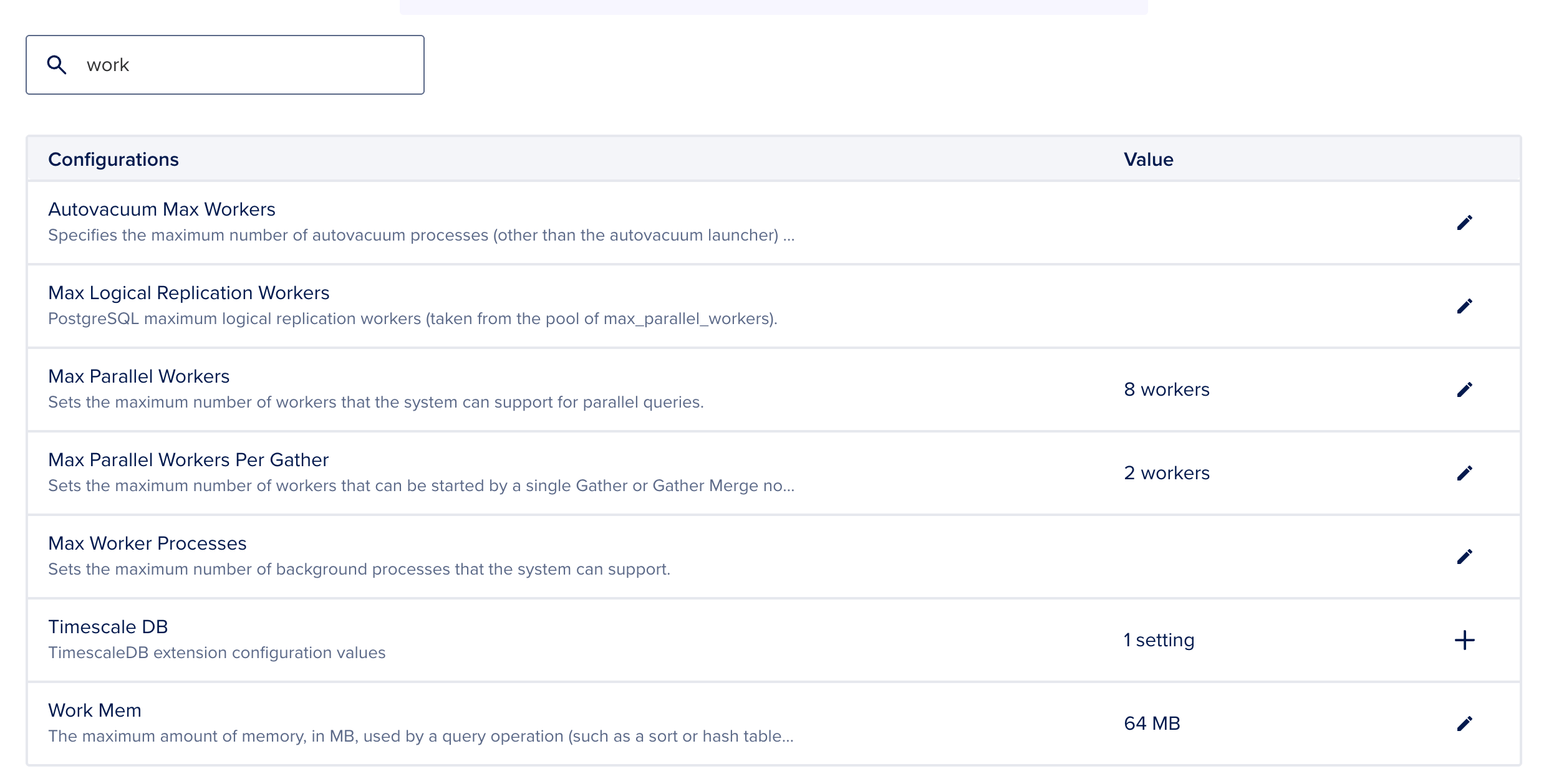
Recommended starting values for an analytics-focused cluster:
| Parameter | Recommended Value | Effect |
|---|---|---|
work_mem |
256MB | Allocates memory per hash operation; reduces disk spill for snowflake multi-join queries |
max_parallel_workers_per_gather |
4 | Enables parallel sequential scans on large fact tables |
enable_hashjoin |
on | Keeps hash join plans enabled; should remain on for analytics workloads |
ALTER SYSTEM is not available on DigitalOcean Managed PostgreSQL. Configure these parameters through the control panel under Settings > Advanced Configurations or via the DigitalOcean API. Setting work_mem too high on shared clusters can cause out-of-memory conditions under concurrent load. Test with session-level overrides first: SET work_mem = '256MB';
For a session-level override before running a specific analytics query:
SET work_mem = '256MB';
This applies only to the current connection and is compatible with PgBouncer in session pooling mode.
Applying the Star or Snowflake Schema with psql or pgAdmin
After connecting to your managed cluster, apply the DDL from the previous sections using psql. If you need to set up a PostgreSQL client, see How To Install and Use PostgreSQL on Ubuntu 22.04 for connection instructions.
psql "postgresql://doadmin:<password>@<cluster-host>:25060/analytics?sslmode=verify-full&sslrootcert=/path/to/ca-certificate.crt" \
    -f star_schema.sql
For pgAdmin, open the Query Tool, paste each DDL block, and execute. Create a dedicated analytics database before running schema DDL to keep analytics tables isolated from application databases on the same cluster.
Table Partitioning and Schema Interaction
Range partitioning on date_key is compatible with both star and snowflake schemas and is the standard approach for fact tables that grow beyond 50 million rows. Partition the fact table by year or quarter using PARTITION BY RANGE:
CREATE TABLE fact_order_items (
    order_item_key  BIGINT GENERATED BY DEFAULT AS IDENTITY,
    order_id        INTEGER       NOT NULL,
    date_key        INTEGER       NOT NULL,
    product_key     INTEGER       NOT NULL,
    customer_key    INTEGER       NOT NULL,
    quantity        INTEGER       NOT NULL,
    unit_price      NUMERIC(10,2) NOT NULL,
    discount        NUMERIC(5,2)  NOT NULL DEFAULT 0,
    revenue         NUMERIC(12,2) NOT NULL
) PARTITION BY RANGE (date_key);

CREATE TABLE fact_order_items_2024
    PARTITION OF fact_order_items
    FOR VALUES FROM (20240101) TO (20250101);

CREATE TABLE fact_order_items_2025
    PARTITION OF fact_order_items
    FOR VALUES FROM (20250101) TO (20260101);
A BRIN index on date_key within each partition reduces index size further because BRIN indexes are built per partition and each partition has a narrower value range than the full table. Both star and snowflake schemas benefit equally from partitioning because the fact table structure is identical in both patterns. The dimension tables are not partitioned.
DigitalOcean Managed PostgreSQL supports declarative partitioning without superuser access. Create partition tables using psql or pgAdmin connected to the cluster as the doadmin user.
Connection Pooling Considerations with PgBouncer
DigitalOcean Managed PostgreSQL includes a built-in PgBouncer connection pooler. For analytics workloads, use session pooling mode rather than transaction pooling mode.
Transaction pooling returns connections to the pool after each statement, which is incompatible with session-level SET work_mem overrides and with prepared statement caching used by some BI tools. Create a dedicated connection pool for analytics connections in the Managed Database control panel under Connection Pools, and configure it with session mode and a pool size appropriate for your concurrent analytics query load.
Normalization vs Denormalization: The Core Trade-off
Neither pattern is unconditionally better. The right choice depends on how often dimension attributes change, how many fact tables share those dimensions, and what your ETL pipeline can reliably produce at load time.
When Denormalization Serves Analytics Workloads
Denormalization reduces the number of tables a query must touch to produce a result. For read-heavy OLAP workloads where data is loaded in nightly or hourly batches and rarely updated in place, storing redundant attribute values in flat dimension tables is usually an acceptable cost for the query simplicity it provides.
A flat dim_products table also benefits BI tools with limited query optimization. Some spreadsheet-based connectors and embedded analytics libraries generate single-join aggregation queries and cannot traverse multi-table hierarchies without manual configuration.
When Normalization Reduces Long-Term Storage and Update Costs
Normalization provides the most benefit when dimension attributes have low cardinality and high repetition. In a larger deployment, if dim_products has 100,000 rows and category_name takes one of 5 possible values, storing the full string 100,000 times is wasteful compared to 5 rows in product_category and an integer foreign key in dim_products.
The update cost advantage is significant with SCD Type 1 patterns, where attribute changes overwrite historical values. A single UPDATE to one row in product_category is cheaper and less error-prone than a batch UPDATE across 10,000 rows in dim_products.
Hybrid Approaches: Partially Normalized Dimensions
A hybrid schema normalizes high-cardinality, frequently updated dimension attributes while keeping low-cardinality, stable attributes flat. You might normalize product_category and product_subcategory into separate tables because they change occasionally and are shared across multiple fact tables, while keeping customer address attributes flat in dim_customers because addresses are unique per customer and rarely grouped in analytical queries.
This approach is common in production PostgreSQL data warehouses where different dimensions have different operational characteristics and update frequencies.
Choosing Between Star and Snowflake Schema: A Decision Framework
Use the checklist below when starting a new analytics project or evaluating whether an existing schema is causing more operational friction than it solves.
The decision rule in one sentence: If your most frequent BI queries traverse a dimension hierarchy on a fact table above 50 million rows, a star schema will be measurably faster than the equivalent snowflake schema on the same managed PostgreSQL cluster. Below 10 million rows, the difference is dominated by index quality and work_mem configuration, not schema choice.
Decision Criteria Checklist
- Dimension update frequency: if dimension attributes change more than monthly, favor snowflake to reduce update anomalies.
- Fact table row count: below 10 million rows, the query performance difference is usually negligible with proper indexing; above 50 million rows, benchmark both schemas with representative queries before committing.
- BI tool SQL generation: if your tool generates SQL automatically, verify it produces efficient multi-join queries; star schemas are safer for tools with limited query optimization.
- Shared dimensions: if the same lookup data appears in multiple fact tables, normalizing it into shared dimension tables prevents attribute divergence.
- ETL pipeline maturity: denormalization requires a reliable, tested ETL process; if your pipeline is early-stage, start with snowflake and denormalize later once the pipeline is stable.
- Team SQL proficiency: snowflake schemas require more complex query authoring; if your analysts are less experienced with multi-table joins, star schemas reduce friction.
Signals That Indicate You Should Migrate from One Schema to the Other
Migrate from star to snowflake when dimension table updates are becoming expensive due to high-cardinality redundant attributes, or when multiple fact tables need to share dimension data and synchronization is failing.
Migrate from snowflake to star when EXPLAIN ANALYZE output consistently shows join overhead as the bottleneck on your most frequent BI reports, and when your ETL pipeline can reliably denormalize dimensions before loading.
Migrating Between Schemas Without Downtime
Use the view-swap pattern to migrate from a snowflake schema to a star schema without taking the database offline or blocking reads. The full procedure with SQL is covered in the FAQ answer for migration, but the operational sequence is:
- Create a denormalized view of the snowflake dimension hierarchy.
- Validate the view returns correct row counts and column values against your existing queries.
- Create the new physical star schema table using the same column names and types as the view.
- Backfill the table from the view inside a transaction.
- In a single transaction, rename the original tables and swap in the new star schema table.
- Drop the normalized lookup tables after confirming all queries route correctly to the new table.
The view acts as a contract between the old schema and the new one: queries continue running against the view during the migration window, and the physical swap is instant at the DDL level.
Frequently Asked Questions
Q: Is star schema always faster than snowflake schema in PostgreSQL?
Not always. The performance difference depends on join count, table sizes, work_mem configuration, and index coverage. A star schema requires fewer hash join operations than the equivalent snowflake query for the same fact table, so it tends to be faster for hierarchy-traversing aggregations. At low row counts the difference is often negligible. The PostgreSQL query planner optimizes hash join sequences based on statistics collected by ANALYZE; stale statistics cause more performance degradation than the schema choice itself, so running ANALYZE after bulk loads has more impact on query latency than schema selection at small scale.
Q: Does PostgreSQL handle snowflake schema joins efficiently at scale?
At high row counts with insufficient work_mem, the planner starts spilling intermediate hash tables to disk. The more joins your snowflake query requires, the more likely this is to happen, and the larger the performance gap relative to an equivalent star schema query. Increasing work_mem to 128-256 MB on DigitalOcean Managed PostgreSQL reduces disk spill and narrows the gap; the exact improvement depends on your fact table size, join count, and concurrency level. Run ANALYZE after loading new dimension data. Stale statistics cause the planner to pick the wrong join order, and that has more impact on snowflake queries than on star schema queries because there are more joins to get wrong.
Q: Can I use both star and snowflake patterns in the same PostgreSQL database?
Yes. Different subject areas in the same database can use different schema patterns. A sales subject area might use a star schema with a flat dim_products table, while an inventory subject area uses a snowflake schema with normalized product_subcategory and product_category tables. The product_category table in the snowflake schema can serve as a shared dimension by adding a foreign key from the star schema’s dim_products to it, combining both patterns in a hybrid design. This is a practical approach when different subject areas have different query access patterns and update frequencies.
Q: How does storage cost differ between star and snowflake schemas on DigitalOcean Managed PostgreSQL?
For a concrete estimate: dim_products with 20,000 rows storing two VARCHAR(100) attributes uses roughly 4 MB for those columns. Normalizing those attributes into product_category (5 rows) and product_subcategory (2,800 rows) reduces that to under 50 KB. The fact table stores integer foreign keys in both schemas, so the storage difference is in the dimension tables, not in fact_order_items. On managed PostgreSQL where storage is billed by the gigabyte, snowflaking dimension tables typically saves less than 1% of total storage for a schema with a properly designed fact table. Storage savings are more significant when dimension tables have high row counts (above 500,000) with multiple low-cardinality attributes.
Q: What PostgreSQL index types work best for fact tables in a star schema?
BRIN indexes work well for date_key columns in append-only fact tables where row values are correlated with insertion order. A BRIN index on date_key is orders of magnitude smaller than a B-tree index on the same column and has lower maintenance overhead during bulk inserts. For foreign key columns such as product_key and customer_key, B-tree indexes are useful when queries filter selectively on those keys and when the planner chooses nested-loop or merge joins. Covering indexes using the INCLUDE clause are effective for queries that aggregate revenue grouped by date_key and product_key: the planner can satisfy the query from the index without accessing the heap, which reduces I/O significantly on large fact tables.
Q: How do I migrate from a snowflake schema to a star schema in PostgreSQL without downtime?
Follow these steps to migrate without downtime:
- Create a denormalized view of the snowflake dimension.
- Validate the view against your existing queries.
- Create the new physical star schema table.
- Backfill the table from the view.
- In a single transaction, rename the old table and swap in the new one.
- Drop the normalized tables after verifying all queries route correctly.
For step 1, create a denormalized view of the snowflake dimension:
CREATE VIEW v_dim_products_flat AS
SELECT dp.product_key, dp.product_id, dp.product_name,
       ps.subcategory_name, pc.category_name
FROM dim_products        dp
JOIN product_subcategory ps ON dp.subcategory_key = ps.subcategory_key
JOIN product_category    pc ON ps.category_key    = pc.category_key;
For step 3, create the physical star schema table:
CREATE TABLE dim_products_star (
    product_key       INTEGER GENERATED BY DEFAULT AS IDENTITY PRIMARY KEY,
    product_id        INTEGER      NOT NULL UNIQUE,
    product_name      VARCHAR(255) NOT NULL,
    subcategory_name  VARCHAR(100) NOT NULL,
    category_name     VARCHAR(100) NOT NULL
);
For step 4, backfill from the view:
INSERT INTO dim_products_star
SELECT product_key, product_id, product_name, subcategory_name, category_name
FROM v_dim_products_flat;
After backfilling, validate row counts match between v_dim_products_flat and dim_products_star before proceeding to the swap in step 5.
Q: Does DigitalOcean Managed PostgreSQL support the configuration changes needed for analytics workloads?
Yes. The following parameters are configurable through the DigitalOcean control panel under Settings > Advanced Configurations, or via the DigitalOcean API:
work_mem: controls memory per sort or hash operation; increasing this reduces disk spill for multi-join snowflake queries.max_parallel_workers_per_gather: controls parallel workers used for sequential scans and aggregations; increasing from the default of 2 to 4 or 8 on larger clusters reduces scan time on large fact tables.enable_hashjoin: set toonby default; controls whether the planner considers hash join plans.
Parameters not configurable on managed PostgreSQL include shared_buffers (set automatically based on cluster size) and superuser-only parameters. max_connections is configurable within plan limits.
Q: What is the difference between a snowflake schema and third normal form (3NF) in a data warehouse?
Third normal form (3NF) is a normalization standard designed for transactional databases to eliminate update anomalies in operational systems. A snowflake schema borrows the same structural principle but applies it selectively to dimension tables in an analytical context. In a strict 3NF transactional schema, every non-key attribute must depend only on the primary key of its table. In a snowflake schema, the fact table is intentionally not in 3NF: it stores additive measures like revenue and quantity alongside multiple foreign keys, because those measures depend on the combination of keys, not a single key. The dimension hierarchies are normalized, but the overall schema is not in 3NF. The goal of snowflaking is not full normalization but controlled normalization of specific attribute hierarchies that have update anomaly risks or storage overhead worth addressing.
Conclusion
Star and snowflake schemas are not competing standards so much as two points on a trade-off curve between query simplicity and data model integrity. This tutorial walked through both patterns in full, from DDL to EXPLAIN ANALYZE output on 2.7 million fact rows, covering how the additional hash join operations in a snowflake query affect query plan shape, how to address that with index and configuration choices, and what conditions in your own workload should push you toward one schema or the other.
With these DDL examples and the decision framework in the final section, you can provision a DigitalOcean Managed PostgreSQL cluster, apply the schema that fits your workload, and configure work_mem, connection pooling, and indexes for analytics query performance. The comparison table and checklist provide a repeatable process for evaluating schema choices as data volume and team requirements evolve.
As a concrete next step, run the EXPLAIN ANALYZE queries from this tutorial on both schemas, then add two more representative reports: a single-dimension aggregation and a filtered multi-dimension GROUP BY with a date range predicate. Compare planning time and execution time for each pair. The results will confirm whether your workload sits in the regime where schema choice drives performance or where index quality and work_mem configuration are the dominant factors. To add a natural language query layer on top of your analytics schema, DigitalOcean AI Platform supports text-to-SQL generation against a connected PostgreSQL schema, letting analysts query both schema types without writing SQL directly.
Thanks for learning with the DigitalOcean Community. Check out our offerings for compute, storage, networking, and managed databases.
About the author
Building future-ready infrastructure with Linux, Cloud, and DevOps. Full Stack Developer & System Administrator. Technical Writer @ DigitalOcean | GitHub Contributor | Passionate about Docker, PostgreSQL, and Open Source | Exploring NLP & AI-TensorFlow | Nailed over 50+ deployments across production environments.
Still looking for an answer?
This textbox defaults to using Markdown to format your answer.
You can type !ref in this text area to quickly search our full set of tutorials, documentation & marketplace offerings and insert the link!
 This work is licensed under a Creative Commons Attribution-NonCommercial- ShareAlike 4.0 International License.
Become a contributor for community
Get paid to write technical tutorials and select a tech-focused charity to receive a matching donation.

DigitalOcean Documentation
Full documentation for every DigitalOcean product.

Resources for startups and AI-native businesses
The Wave has everything you need to know about building a business, from raising funding to marketing your product.
The developer cloud
Scale up as you grow — whether you're running one virtual machine or ten thousand.

Start building today
From GPU-powered inference and Kubernetes to managed databases and storage, get everything you need to build, scale, and deploy intelligent applications.
