AI Technical Writer

YOLO26 is a modern deep learning model designed for real-time object detection tasks. It extends the YOLO (You Only Look Once) family of models by introducing anchor-free and NMS-free detection, enabling faster inference and simpler deployment pipelines. With improved architecture and optimized training strategies, YOLO26 achieves strong performance across edge devices, cloud GPUs, and large-scale computer vision systems.
In this tutorial, you’ll learn how YOLO26 works, how it compares to earlier YOLO models, and how to install, finetune, and infer it for real-world object detection tasks.
We begin by setting up the YOLO26 model and running inference with a pretrained version to understand how the model detects objects. Next, we fine-tune the YOLO26n model on the SKU-110K dataset, a large retail shelf dataset containing densely packed products commonly found in stores.
Fine-tuning the model on this dataset helps it learn to accurately detect and count retail items that are visually similar and closely positioned, which is essential for real-world applications such as automated inventory monitoring, retail shelf analytics, and product availability tracking. To accelerate training, the model is trained on DigitalOcean GPU Droplets, which provide high-performance compute and large memory capacity for deep learning workloads.
Finally, we built a simple Gradio application that allows users to upload an image and run YOLO26 inference through a web interface, displaying bounding boxes around detected items along with product counts. This end-to-end workflow demonstrates how to train, deploy, and interact with a YOLO26 object detection system for practical retail use cases.
Key Takeaways
- YOLO26 is a modern real-time object detection model designed for speed and simplicity.
- The model introduces anchor-free and NMS-free detection, reducing inference complexity.
- YOLO26 supports multiple tasks, including object detection and instance segmentation.
- Cloud GPU environments allow scalable training and deployment workflows.
- Compared with YOLOv11 and RF-DETR, YOLO26 provides a strong balance of accuracy, speed, and ease of deployment.
What Is YOLO26?
YOLO26 is a convolutional neural network (CNN) designed for real-time object detection. Like previous YOLO models, it processes an entire image in a single forward pass and predicts bounding boxes, object classes, and confidence scores simultaneously.
However, YOLO26 introduces several architectural changes:
The architecture of YOLO26 is designed around simplicity, deployment efficiency, and training innovation to improve real-world usability. Unlike earlier YOLO models that rely on post-processing steps such as Non-Maximum Suppression (NMS), YOLO26 adopts a native end-to-end design that produces predictions directly from the network, reducing latency and simplifying deployment pipelines. This approach, first introduced in YOLOv10, enables faster inference and more efficient integration into production systems. YOLO26 also introduces the MuSGD optimizer, a hybrid optimization method inspired by advances in large language model training, which improves training stability and accelerates convergence.
The optimizer has been inspired by Moonshot AI’s Kimi K2 in LLM training.
In addition, the model incorporates task-specific optimizations for various computer vision tasks, including enhanced loss functions for semantic segmentation, multi-scale prototype modules for segmentation accuracy, Residual Log-Likelihood Estimation (RLE) for improved pose estimation, and optimized decoding techniques for oriented bounding box detection. Together, these architectural improvements enable YOLO26 to achieve stronger performance on small objects, faster CPU inference, and more efficient deployment, making it a practical object detection solution for modern AI applications and resource-constrained environments.
These improvements make YOLO26 well-suited for applications such as:
- autonomous driving systems
- retail shelf monitoring
- industrial defect detection
- edge device object detection
- video surveillance systems
YOLO26 is up to 43% faster on CPUs compared to previous generations, making it ideal for edge deployment.
YOLO26 Model Variants and Performance Benchmarks
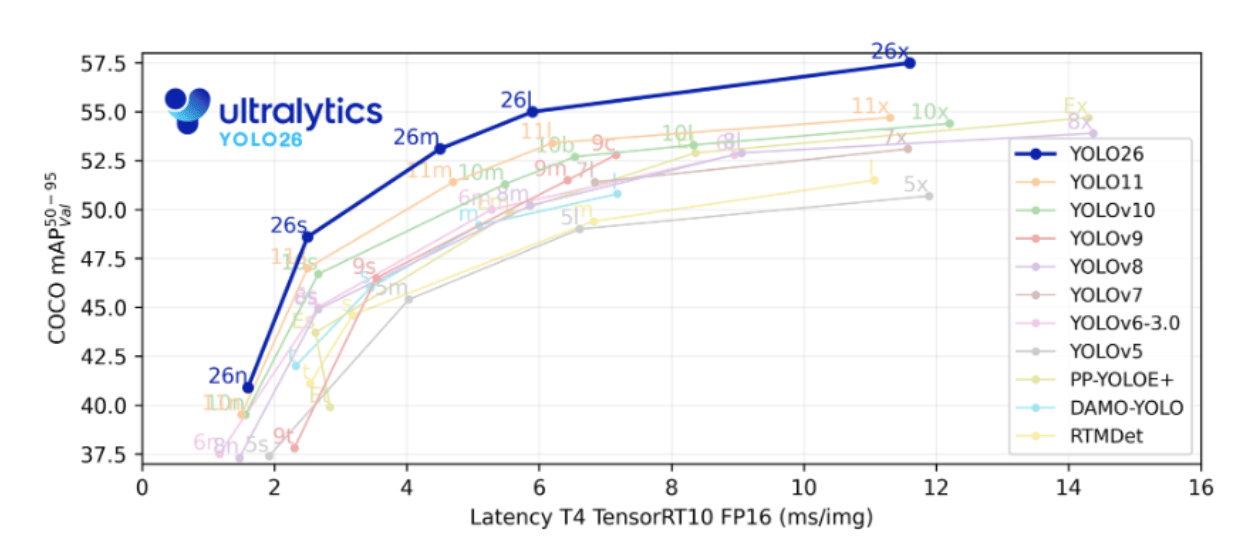
YOLO26 is available in multiple variants designed for different hardware capabilities.
| Model Variant | Parameters | mAP (COCO) | Latency (ms) | Use Case |
|---|---|---|---|---|
| YOLO26-Nano | ~2.4M | ~40.9 | ~2.4 | Edge devices |
| YOLO26-Small | ~10M | ~48.5 | ~4.7 | Embedded GPUs |
| YOLO26-Medium | ~20M | ~52.5 | ~7.8 | Real-time inference |
| YOLO26-Large | ~25M | ~54.4 | ~11.9 | High-accuracy workloads |
| YOLO26-XLarge | ~55M | ~57.5 | ~17.2 | Cloud GPU training |
YOLO26 vs YOLO11: Key Differences and Performance Comparison
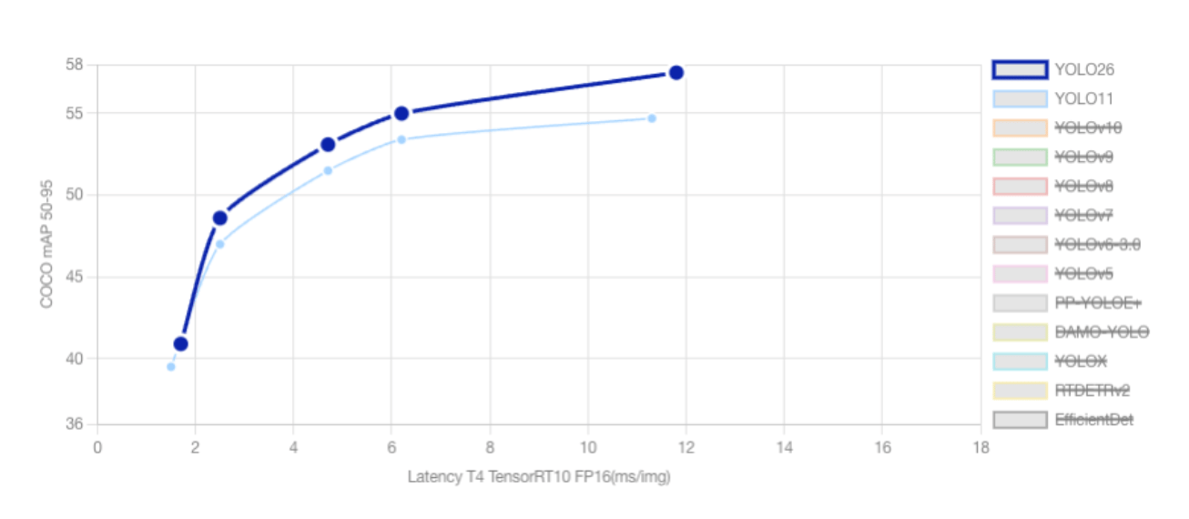
As the YOLO family continues to add new models, each of the new versions introduces architectural improvements aimed at improving accuracy, speed, and deployment efficiency. YOLO11 established a strong baseline for real-time object detection and multi-task computer vision workloads, while YOLO26 represents a significant step forward, especially for edge computing and low-power environments.
Architectural Improvements
One of the most significant differences between the two models is the end-to-end NMS-free architecture introduced in YOLO26. Traditional YOLO models, including YOLO11, rely on Non-Maximum Suppression (NMS) to remove duplicate bounding boxes after the model makes predictions. YOLO26 eliminates this step entirely by producing final predictions directly from the network. This reduces latency, simplifies deployment pipelines, and improves consistency when running on edge devices.
Another key improvement in YOLO26 is the removal of Distribution Focal Loss (DFL). While YOLO11 uses DFL to refine bounding box predictions, this technique requires complex softmax operations that are often inefficient on low-power hardware. By removing DFL, YOLO26 simplifies the architecture and improves compatibility with embedded systems and edge accelerators.
Training Innovations
YOLO26 introduces a new optimization method called MuSGD, a hybrid of Stochastic Gradient Descent (SGD) and Muon-inspired optimization strategies. This optimizer improves training stability and convergence speed while maintaining lower memory usage compared to more complex training pipelines.
In addition, YOLO26 includes new loss functions designed to improve performance in challenging scenarios such as small object detection. Techniques such as ProgLoss and Scale-Targeted Attention Loss (STAL) help the model detect small or distant objects more accurately, which is particularly useful in applications like aerial imagery and drone-based monitoring.
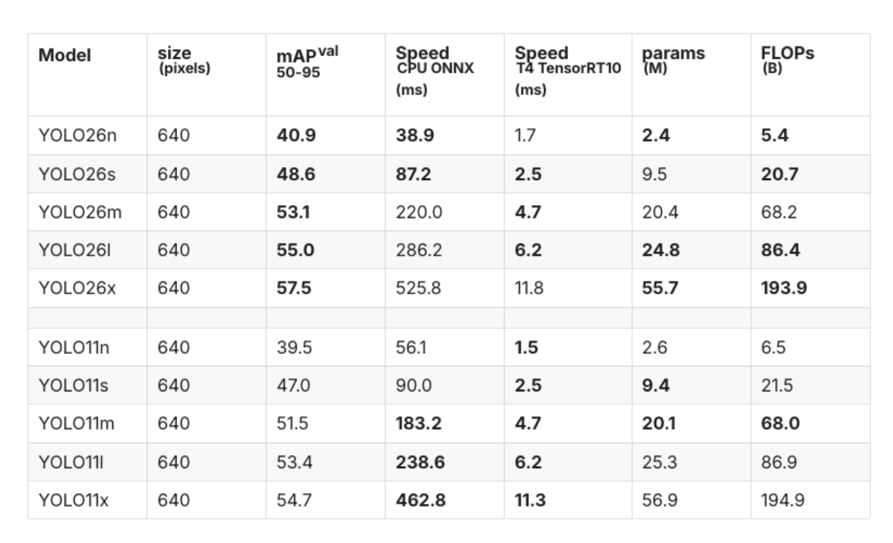
Performance Comparison
The improvements in YOLO26 translate directly into measurable performance gains. For example, the YOLO26 nano (YOLO26n) model achieves approximately 40.9 mAP (50–95) on validation datasets while delivering significantly faster CPU inference compared to YOLO11.
| Model | mAP (50–95) | CPU ONNX Speed (ms) | Parameters (M) |
|---|---|---|---|
| YOLO26n | 40.9 | 38.9 | 2.4 |
| YOLO11n | 39.5 | 56.1 | 2.6 |
This represents roughly a 31% improvement in CPU inference speed, demonstrating YOLO26’s strong focus on edge-device performance.
Task Support and Versatility
Both YOLO26 and YOLO11 support multiple computer vision tasks within the Ultralytics framework, including:
- Object Detection
- Instance Segmentation
- Pose Estimation
- Image Classification
- Oriented Bounding Box Detection
However, YOLO26 introduces additional improvements for specialized tasks. For instance, its multi-scale prototype modules improve instance segmentation quality, while Residual Log-Likelihood Estimation (RLE) enhances keypoint accuracy for pose estimation. YOLO26 also includes improved decoding strategies for oriented bounding box detection, making it suitable for applications such as satellite imagery analysis.
When YOLO11 May Still Be Useful
Although YOLO26 offers several advantages, YOLO11 remains a capable model and may still be used in certain scenarios. For example, existing production pipelines built around older YOLO architectures may rely on NMS-based detection outputs, making migration more complex. Additionally, YOLO11 may still be used as a baseline model in academic research where consistency with earlier benchmarks is required.
Overall, YOLO26 represents a major advancement in the YOLO ecosystem by combining higher accuracy, faster inference, and improved deployment efficiency, making it one of the most practical real-time object detection models available today.
Conceptual Architecture
YOLO26 processes images through several stages:
Input Image
     │
     ▼
CNN Backbone
     │
     ▼
Feature Pyramid Network
     │
     ▼
Detection Head
     │
     ▼
Bounding Boxes + Classes
Because YOLO26 uses NMS-free detection, predictions can be processed faster without additional filtering steps.
Prerequisites
Before installing YOLO26, ensure your environment includes:
- Python 3.9 or later
- PyTorch
- CUDA-enabled GPU (recommended)
- pip package manager
- Recommended: NVIDIA GPU for large dataset training
For development workflows, many practitioners use Jupyter Notebook for experimentation. If you need a setup guide, refer to DigitalOcean’s tutorial on setting up a Python notebook environment.
How to Install YOLO26 with Ultralytics
YOLO26 is integrated into the Ultralytics framework, which simplifies training and inference.
Step 1: Install Dependencies
We will first install all the necessary libraries, such as OpenCV, matplotlib.
pip install ultralytics opencv-python matplotlib
Step 2: Import the libraries and Verify Installation
Import the necessary libraries and verify that everything is installed correctly.
import cv2
import matplotlib.pyplot as plt
from ultralytics import YOLO
print("Ultralytics installed successfully")
Step 3: Download a YOLO26 Model
# Load a COCO-pretrained YOLO26n model
model = YOLO("yolo26n.pt")
The n variant refers to the Nano model, optimized for speed and edge deployment.
Running Inference with a Pretrained YOLO26 Model
Inference allows you to detect objects using a pretrained model.
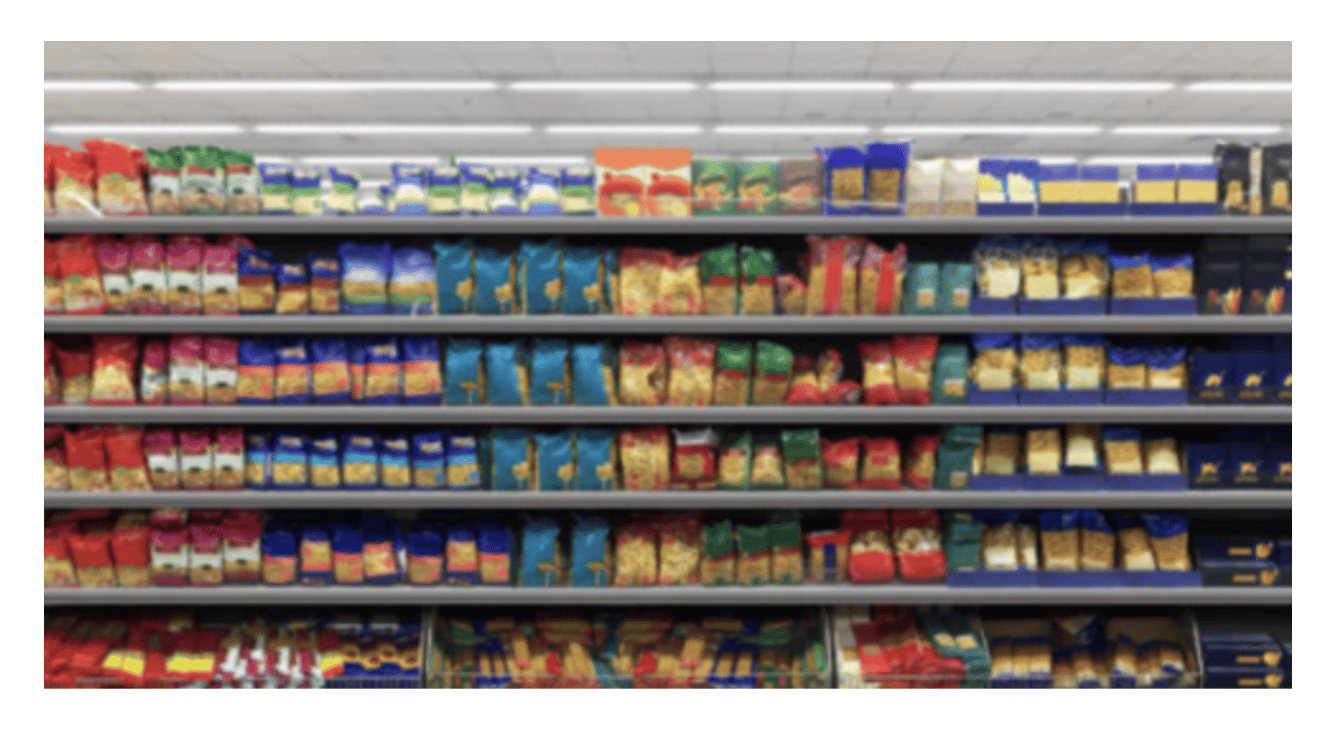
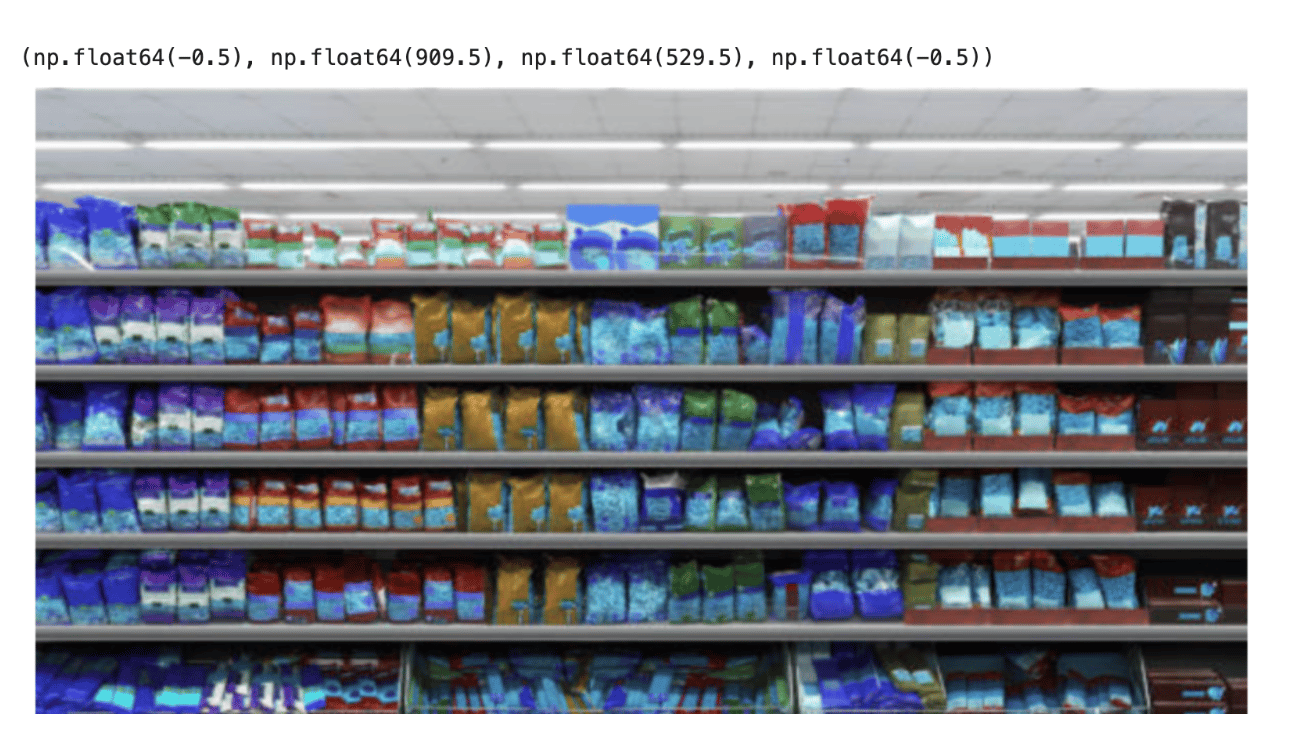
Load an image to run inference using the Image
image_path = "image1.jpeg"

image = cv2.imread("image1.jpeg")

if image is None:
   print(f"Error: Could not load image from {image_path}. Please make sure the file exists and the path is correct.")
else:
   image_rgb = cv2.cvtColor(image, cv2.COLOR_BGR2RGB)
   plt.imshow(image_rgb)
   plt.axis("off")
Running Inference with the Pretrained YOLO26 Model
We will use this image and the loaded model to run detection on it and observe how the model behaves. The loaded model is trained on the COCO dataset, and it is clear that it will not produce accurate results.
results = model(image_path)
result = results[0]

annotated_image = result.plot()

plt.figure(figsize=(10,8))
plt.imshow(annotated_image)
plt.axis("off")
Also, the output images containing predicted bounding boxes will be saved to:
runs/detect/predict
Since the YOLO26n model was trained on the COCO dataset and not fine-tuned on retail shelf data, it fails to correctly identify individual store products and instead produces generalized detections or inaccurate bounding regions across the shelf items.
Fine-Tuning YOLOv26n for Retail Shelf Detection Using the SKU-110K Dataset
The SKU-110K dataset is a large-scale collection of densely packed retail shelf images created to support research in object detection. Developed by Eran Goldman et al., the dataset includes more than 110,000 unique stock-keeping unit (SKU) instances, where products are tightly arranged on store shelves. Many of the items appear visually similar or nearly identical, and they are often placed very close to one another, making the dataset particularly challenging for object detection models.
This fine-tuned model can be used for tasks such as:
- Retail shelf monitoring
- Automated inventory counting
- Out-of-stock detection
Dataset Structure
dataset/
 ├── images
 │   ├── train
 │   └── val
 ├── labels
 │   ├── train
 │   └── val
 └── data.yaml
Fine-Tuning YOLO26 Using DigitalOcean GPU Droplet
Fine-tuning a deep learning model such as YOLO26 requires significant computational resources, especially when training on large datasets like SKU-110K. While it is possible to train the model on a local machine using a CPU or a smaller GPU, the training process can take considerably longer depending on the dataset size and model configuration. Using a DigitalOcean GPU Droplet is not mandatory for training YOLO26, but it can significantly accelerate the process.
from ultralytics import YOLO
#Load the model

model = YOLO("yolo26n.pt") #load the pretrained model

# Train the model
results = model.train(data="SKU-110K.yaml", epochs=100, imgsz=640)
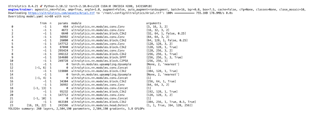
The training process can take a considerable amount of time, depending on the computing resources available. In this tutorial, the model was trained using the H200 GPU available on DigitalOcean GPU Droplets. The H200 provides high-performance GPU acceleration with large memory capacity, which significantly speeds up deep learning workloads such as training object detection models.
Once the model is trained, the trained weights will be saved to:
/root/runs/detect/train
YOLO26 also supports object detection, which predicts both bounding boxes and segmentation masks.
Running Inference using the Finetuned YOLO26 Model
We will use the model on the same image that we passed earlier to the COCO-trained model to check how the model behaves.
Once the training process is complete, the best-performing model checkpoint is saved in the training directory. In this case, the trained YOLOv26n model is stored at runs/detect/train/weights/best.pt. This file contains the model weights that achieved the highest validation performance during training. We can load this trained model and use it for inference to detect products in new images.
# Load trained model
model = YOLO("runs/detect/train/weights/best.pt")

# Run inference on an image
results = model("image1.jpeg", save=True)

# Print results
print(results)
result = results[0]

annotated_image = result.plot()

plt.figure(figsize=(10,8))
plt.imshow(annotated_image)
plt.axis("off")
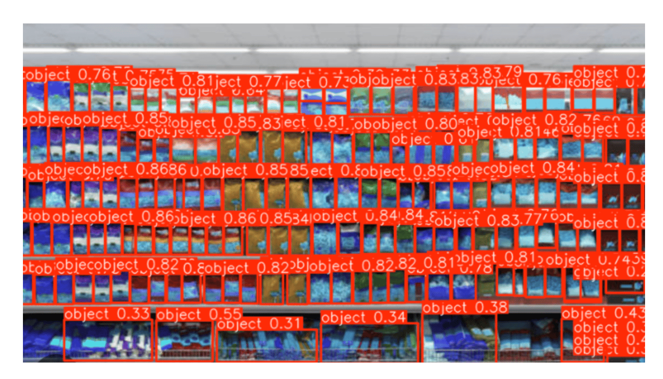
Now we can see that the trained model has clearly identified the objects on the shelf.
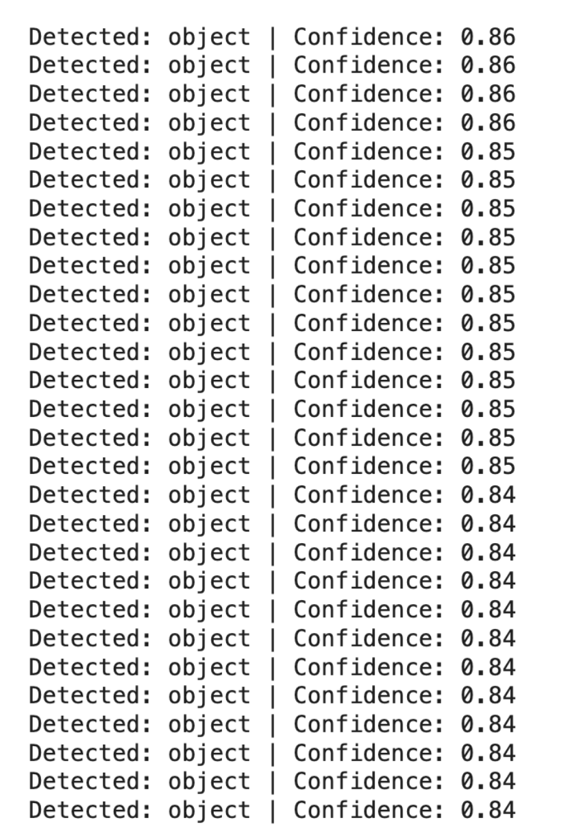
for box in result.boxes:
   class_id = int(box.cls[0])
   confidence = float(box.conf[0])
   label = model.names[class_id]

   print(f"Detected: {label} | Confidence: {confidence:.2f}")
from collections import Counter

detections = []

for box in result.boxes:
   class_id = int(box.cls[0])
   label = model.names[class_id]
   detections.append(label)

counts = Counter(detections)

print("Product Counts:")
for item, count in counts.items():
   print(f"{item}: {count}")
Product Counts:
object: 177
This code:
- Reads all detected objects from YOLO predictions
- Identifies their class labels
- Counts how many times each object appears
- Prints the number of detected items per class
Building a Gradio App for YOLO26 Image Detection and Product Counting
Install the gradio package.
pip install gradio
import gradio as gr
from ultralytics import YOLO
import cv2
import pandas as pd
# Load trained YOLO model
model = YOLO("runs/detect/train2/weights/best.pt")
def detect_objects(image):
# Run inference
results = model(image)
# Annotated image with bounding boxes
annotated_img = results[0].plot()
# Count total objects
total_objects = len(results[0].boxes)
# Count objects per class
class_counts = {}
for box in results[0].boxes:
cls_id = int(box.cls)
class_name = model.names[cls_id]
if class_name not in class_counts:
class_counts[class_name] = 0
class_counts[class_name] += 1
# Convert class counts to table
df = pd.DataFrame(list(class_counts.items()), columns=["Class", "Count"])
return annotated_img, total_objects, df
app = gr.Interface(
fn=detect_objects,
inputs=gr.Image(type="numpy", label="Upload Image"),
outputs=[
gr.Image(label="Predicted Image with Bounding Boxes"),
gr.Number(label="Total Objects Detected"),
gr.Dataframe(label="Detected Class Counts")
],
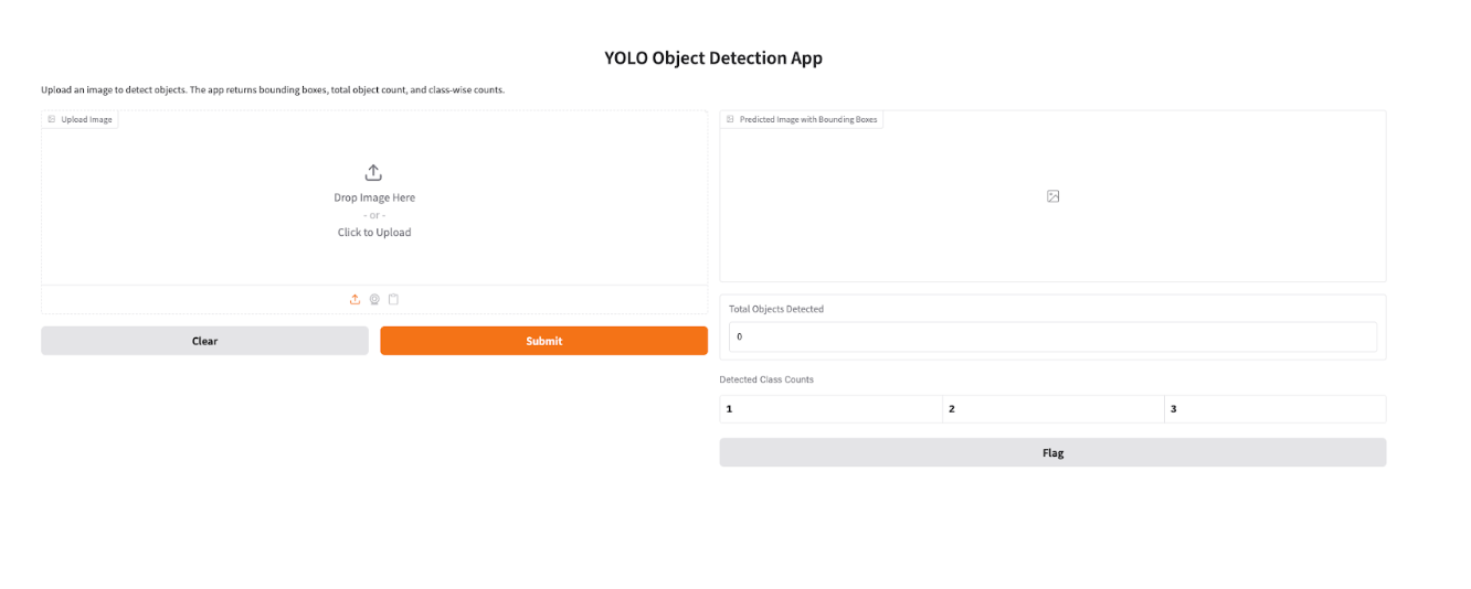
title="YOLO Object Detection App",
description="Upload an image to detect objects. The app returns bounding boxes, total object count, and class-wise counts."
)
app.launch()
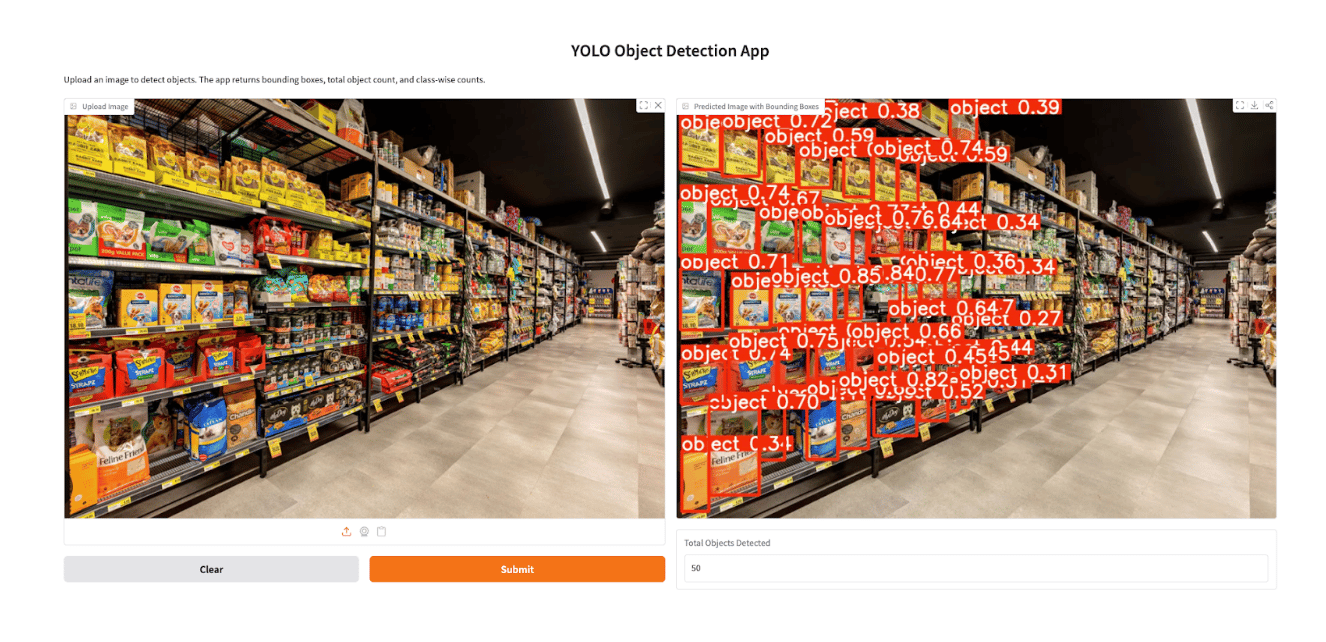
To make the trained YOLO26 model easier to interact with, we can build a simple web interface using Gradio. Gradio allows you to quickly convert models into shareable web applications without requiring complex frontend development. In this example, the Gradio app allows users to upload an image of a retail shelf, run inference using the trained YOLO26 model, and visualize the results with bounding boxes drawn around detected products. Additionally, the application displays the count of each detected product class, making it useful for tasks such as retail inventory monitoring and automated shelf analysis.
Benchmark YOLO26 Model
After training and validating your YOLO26 model, the next step is to evaluate how well it performs under different deployment conditions. Benchmarking allows you to measure the model’s speed, accuracy, and efficiency across various export formats and hardware environments. This is particularly useful when deciding how to deploy your model in production, whether on GPUs, CPUs, or edge devices.
Ultralytics provides a Benchmark mode that automatically evaluates the model using key performance metrics such as mean Average Precision (mAP50–95) and inference time per image. These metrics help determine the balance between detection accuracy and processing speed. Benchmarking also enables developers to compare how the same model performs when exported to different formats like ONNX, TensorRT, or OpenVINO, each optimized for different hardware environments.
For example, the following Python code benchmarks the YOLO26 model on a GPU:
from ultralytics.utils.benchmarks import benchmark

# Benchmark YOLO26 model
benchmark(model="yolo26n.pt", data="coco8.yaml", imgsz=640, half=True)
This command evaluates the model on the specified dataset and reports metrics such as inference latency and detection accuracy. You can also benchmark a specific export format by specifying the format argument:
benchmark(model="yolo26n.pt", data="coco8.yaml", imgsz=640, format="onnx")
Running benchmarks helps you determine the best deployment format for your workload. For instance, exporting the model to ONNX can improve CPU inference performance, while TensorRT often provides significant speed improvements on GPUs. By benchmarking different formats, you can choose the configuration that delivers the optimal balance between performance, cost, and deployment requirements.
FAQ
What is YOLO26?
YOLO26 is a deep learning model designed for real-time object detection. It predicts object classes and bounding boxes directly from images using a single neural network pass.
What is the difference between YOLO11 and YOLO26?
YOLO11 uses anchor-based detection and requires non-maximum suppression post-processing to filter overlapping bounding boxes , while YOLO26 introduces anchor-free and NMS-free detection, simplifying the inference pipeline.
Is YOLO26 better than RF-DETR?
RF-DETR may achieve slightly higher accuracy in some benchmarks, but YOLO26 offers faster inference speeds, making it more suitable for real-time systems.
What is the latest YOLO version?
YOLO26 represents one of the most recent developments in the YOLO family of models, focusing on simplifying detection architecture and improving real-time performance.
Can YOLO26 run on a Raspberry Pi?
Yes. Smaller variants like YOLO26-Nano are designed for low-power device inference and can run on Raspberry Pi or edge AI hardware with optimization.
What is Non-Maximum Suppression (NMS)?
Non-Maximum Suppression (NMS) is a post-processing technique used in object detection models to remove duplicate bounding boxes that refer to the same object. During detection, a model may predict multiple overlapping boxes with different confidence scores for one object. NMS keeps the box with the highest confidence score and suppresses the others that overlap significantly. This ensures that each object is detected with a single, clean bounding box instead of multiple redundant predictions.
What tasks does YOLO26 support beyond object detection?
YOLO26 can also perform:
- instance segmentation
- pose estimation
- image classification
How do I train YOLO26 on a custom dataset?
Training involves preparing images and label files, creating a dataset configuration file (data.yaml), and running the Ultralytics training command.
What GPU is recommended for training YOLO26?
For large datasets, GPUs such as NVIDIA A100 or H100 provide optimal training performance. Smaller models can also be trained on GPUs like the NVIDIA T4.
When to Choose YOLO26
YOLO26 is generally the preferred choice for most new projects, especially when working with:
- Edge and IoT devices
- Real-time robotics systems
- Drone and aerial analytics
- Low-power inference environments
Its NMS-free design and optimized architecture allow it to run faster and more efficiently in latency-sensitive applications.
Conclusion
In this tutorial, we explored how to work with Ultralytics YOLO26 to build a complete object detection workflow from model setup and inference to fine-tuning and deployment. We started by installing YOLO26 and running inference using a pretrained model to understand how the model detects objects using bounding boxes. We then fine-tuned the YOLO26n model on the SKU-110K dataset, which contains densely packed retail shelf images. Training on this dataset allows the model to better recognize retail products that are visually similar and positioned closely together, making it suitable for practical retail applications.
The model was trained on DigitalOcean GPU Droplets powered by the H200 GPU. While GPU infrastructure is not strictly required, using a high-performance GPU significantly reduces training time and enables faster experimentation with hyperparameters and datasets. This makes it easier for developers and machine learning practitioners to iterate on models and achieve better results without being limited by local hardware constraints.
We also demonstrated how to run inference using the trained model and count detected objects in an image. This capability is particularly useful for retail shelf monitoring, automated inventory counting, and product analytics, where identifying and counting products accurately is essential.
Finally, we built a Gradio application that provides a simple web interface for interacting with the trained YOLO26 model. Users can upload an image, visualize detected products with bounding boxes, and view the number of detected items per class. This step highlights how computer vision models can be quickly turned into interactive tools that are easier to use and share.
Overall, YOLO26 introduces several architectural improvements, including end-to-end NMS-free detection, optimized training with the MuSGD optimizer, and improved efficiency for edge environments, thus making it one of the most practical real-time object detection models available today. By combining these capabilities with cloud GPU infrastructure and simple deployment tools like Gradio, developers can build scalable computer vision applications that move efficiently from experimentation to real-world deployment.
Resources
- Ultralytics YOLO26
- Ultralytics YOLO Docs
- Evaluating Object Detection Models Using Mean Average Precision (mAP)
- YOLOv9 Object Detection Features, Benefits, and Use Cases
- A Comprehensive Guide to YOLO NAS: Object Detection with Neural Architecture Search
- How did I train YOLOv12 on a Custom Dataset with GPUs
- YOLO26 Retail Product Detection Git repo
Thanks for learning with the DigitalOcean Community. Check out our offerings for compute, storage, networking, and managed databases.
About the author
With a strong background in data science and over six years of experience, I am passionate about creating in-depth content on technologies. Currently focused on AI, machine learning, and GPU computing, working on topics ranging from deep learning frameworks to optimizing GPU-based workloads.
Still looking for an answer?
This textbox defaults to using Markdown to format your answer.
You can type !ref in this text area to quickly search our full set of tutorials, documentation & marketplace offerings and insert the link!
 This work is licensed under a Creative Commons Attribution-NonCommercial- ShareAlike 4.0 International License.
Become a contributor for community
Get paid to write technical tutorials and select a tech-focused charity to receive a matching donation.

DigitalOcean Documentation
Full documentation for every DigitalOcean product.

Resources for startups and AI-native businesses
The Wave has everything you need to know about building a business, from raising funding to marketing your product.
The developer cloud
Scale up as you grow — whether you're running one virtual machine or ten thousand.

Start building today
From GPU-powered inference and Kubernetes to managed databases and storage, get everything you need to build, scale, and deploy intelligent applications.
