Quantile() function in R - A brief guide

You can generate the sample quantiles using the quantile() function in R.

Hello people, today we will be looking at how to find the quantiles of the values using the quantile() function.

Quantile: In laymen terms, a quantile is nothing but a sample that is divided into equal groups or sizes. Due to this nature, the quantiles are also called as Fractiles. In the quantiles, the 25th percentile is called as lower quartile, 50th percentile is called as Median and the 75th Percentile is called as the upper quartile.

In the below sections, let’s see how this quantile() function works in R.

---

Quantile() function syntax

The syntax of the Quantile() function in R is,

quantile(x, probs = , na.rm = FALSE)

Where,

• X = the input vector or the values
• Probs = probabilities of values between 0 and 1.
• na.rm = removes the NA values.

---

A Simple Implementation of quantile() function in R

Well, hope you are good with the definition and explanations about quantile function. Now, let’s see how quantile function works in R with the help of a simple example which returns the quantiles for the input data.

#creates a vector having some values and the quantile function will return the percentiles for the data.

df<-c(12,3,4,56,78,18,46,78,100)
quantile(df)

Output:

0%   25%   50%   75%   100%
3    12    46    78    100

In the above sample, you can observe that the quantile function first arranges the input values in the ascending order and then returns the required percentiles of the values.

Note: The quantile function divides the data into equal halves, in which the median acts as middle and over that the remaining lower part is lower quartile and upper part is upper quartile.

---

Handle the missing values - ‘NaN’

NaN’s are everywhere. In this data-driven digital world, you may encounter these NaN’s more frequently, which are often called as the missing values. If your data by any means has these missing values, you can end up with getting the NaN’s in the output or the errors in the output.

So, in order to handle these missing values, we are going to use na.rm function. This function will remove the NA values from our data and returns the true values.

Let’s see how this works.

#creates a vector having values along with NaN's

df<-c(12,3,4,56,78,18,NA,46,78,100,NA)
quantile(df)

Output:

Error in quantile.default(df) :
missing values and NaN's not allowed if 'na.rm' is FALSE

Oh, we got an error. If your guess is regarding the NA values, you are absolutely smart. If NA values are present in our data, the majority of the functions will end up in returning the NA values itself or the error message as mentioned above.

Well, let’s remove these missing values using the na.rm function.

#creates a vector having values along with NaN's

df<-c(12,3,4,56,78,18,NA,46,78,100,NA)

#removes the NA values and returns the percentiles
quantile(df,na.rm = TRUE)

Output:

0%  25%  50%  75%  100%
3   12    46   78   100

In the above sample, you can see the na.rm function and its impact on the output. The function will remove the NA’s to avoid the false output.

---

The ‘Probs’ argument in the quantile

As you can see the probs argument in the syntax, which is showcased in the very first section of the article, you may wonder what does it mean and how it works?. Well, the probs argument is passed to the quantile function to get the specific or the custom percentiles.

Seems to be complicated? Dont worry, I will break it down to simple terms.

Well, whenever you use the function quantile, it returns the standard percentiles like 25,50 and 75 percentiles. But what if you want 47th percentile or maybe 88th percentile?

There comes the argument ‘probs’, in which you can specify the required percentiles to get those.

Before going to the example, you should know few things about the probs argment.

Probs: The probs or the probabilities argument should lie between 0 and 1.

Here is a sample which illustrates the above statement.

#creates the vector of values

df<-c(12,3,4,56,78,18,NA,46,78,100,NA)

#returns the quantile of 22 and 77 th percentiles. 
quantile(df,na.rm = T,probs = c(22,77))

Output:

Error in quantile.default(df, na.rm = T, probs = c(22, 77)) : 
  'probs' outside [0,1]

Oh, it’s an error!

Did you get the idea, what happened?

Well, here comes the Probs statement. Even though we mentioned the right values in the probs argument, it violates the 0-1 condition. The probs argument should include the values which should lie in between 0 and 1.

So, we have to convert the probs 22 and 77 to 0.22 and 0.77. Now the input values is in between 0 and 1 right? I hope this makes sense.

#creates a vector of values
df<-c(12,3,4,56,78,18,NA,46,78,100,NA)

#returns the 22 and 77th percentiles of the input values
quantile(df,na.rm = T,probs = c(0.22,0.77))

Output:

 22%       77% 
10.08     78.00 

---

The ‘Unname’ function and its use

Suppose you want your code to only return the percentiles and avoid the cut points. In these situations, you can make use of the ‘unname’ function.

The ‘unname’ function will remove the headings or the cut points ( 0%,25% , 50%, 75% , 100 %) and returns only the percentiles.

Let’s see how it works!

#creates a vector of values
df<-c(12,3,4,56,78,18,NA,46,78,100,NA)
quantile(df,na.rm = T,probs = c(0.22,0.77))

#avoids the cut-points and returns only the percentiles.
unname(quantile(df,na.rm = T,probs = c(0.22,0.77)))

Output:

10.08      78.00

Now, you can observe that the cut-points are disabled or removed by the unname function and returns only the percentiles.

---

The ‘round’ function and its use

We have discussed the round function in R in detail in the past article. Now, we are going to use the round function to round off the values.

Let’s see how it works!

#creates a vector of values
df<-c(12,3,4,56,78,18,NA,46,78,100,NA)
quantile(df,na.rm = T,probs = c(0.22,0.77))

#returns the round off values
unname(round(quantile(df,na.rm = T,probs = c(0.22,0.77))))

Output:

10   78

As you can see that our output values are rounded off to zero decimal points.

---

Get the quantiles for the multiple groups/columns in a data set

Till now, we have discussed the quantile function, its uses and applications as well as its arguments and how to use them properly.

In this section, we are going to get the quantiles for the multiple columns in a data set. Sounds interesting? follow me!

I am going to use the ‘mtcars’ data set for this purpose and also using the ‘dplyr’ library for this.

#reads the data
data("mtcars")
#returns the top few rows of the data
head(mtcars)

#install required paclages
install.packages('dplyr')
library(dplyr)

#using tapply, we can apply the function to multiple groups
do.call("rbind",tapply(mtcars$mpg, mtcars$gear, quantile))

Output:

     0%     25%    50%     75%    100%
3   10.4   14.5   15.5   18.400   21.5
4   17.8   21.0   22.8   28.075   33.9
5   15.0   15.8   19.7   26.000   30.4

In the above process, we have to install the 'dplyr’ package, and then we will make use of tapply and rbind functions to get the multiple columns of the mtcars datasets.

In the above section, we took multiple columns such as ‘mpg’ and the ‘gear’ columns in mtcars data set. Like this, we can compute the quantiles for multiple groups in a data set.

---

Can we visualise the percentiles?

My answer is a big YES!. The best plot for this will be a box plot. Let me take the iris dataset and will try to visualize the box plot which will showcase the percentiles as well.

Let’s roll!

data(iris)
head(iris)

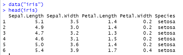
This is the iris data set with top 6 values.

Let’s explore the data with the function named - ‘Summary’.

summary(iris)

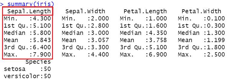
In the above image, you can see the mean, median, 25th percentile(1 st quartile), 75 th percentile(3rd percentile) and min and max values as well. Let’s plot this information through a box plot.

Let’s do it!

#plots a boxplot with labels

boxplot(iris$Sepal.Length,main='The boxplot showing the percentiles',col='Orange',ylab='Values',xlab='Sepal Length',border = 'brown',horizontal = T) 

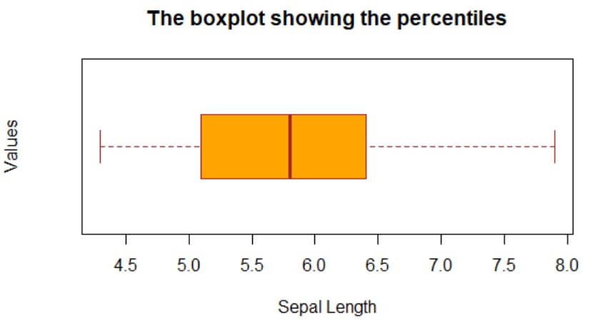
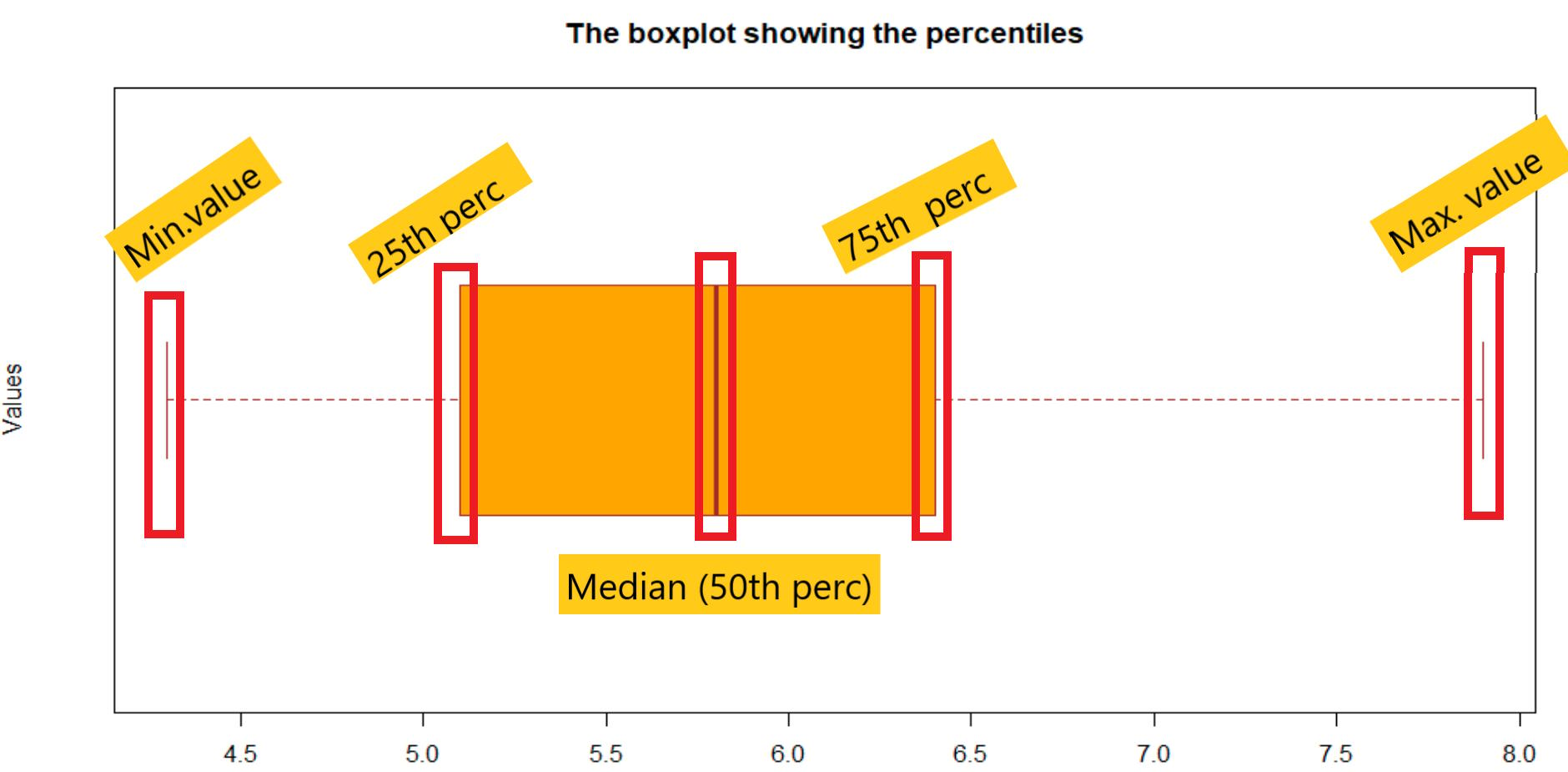
A box plot can show many aspects of the data. In the below figure I have mentioned the particular values represented by the box plots. This will save some time for you and facilitates your understanding in the best way possible.

---

Quantile() function in R - Wrapping up

Well, it’s a longer article I reckon. And I tried my best to explain and explore the quantile() function in R in multiple dimensions through various examples and illustrations as well. The quantile function is the most useful function in data analysis as it efficiently reveals more information about the given data.

I hope you got a good understanding of the buzz around the quantile() function in R. That’s all for now. We will be back with more and more beautiful functions and topics in R programming. Till then take care and happy data analyzing!!!

More study: R documentation.