AI Technical Writer

Introduction
“The past can hurt. But the way I see it, you can either run from it or learn from it.” — Rafiki, The Lion King (1994)
In a world where data drives decisions, learning from the past is more than just wisdom; it’s strategy. From forecasting stock prices to predicting weather conditions and economic trends, the ability to anticipate future values based on historical patterns is at the heart of countless real-world applications. This is where time series analysis becomes essential.
Time series analysis focuses on data points collected or recorded at successive time intervals and understanding this data using certain tools and a few mathematical equations. What makes this type of data unique is its dependency on time; unlike other datasets, the order and timing of each data point are essential.
A foundational method in this field is the Autoregressive (AR) model. AR models operate on a straightforward yet powerful idea: the future value of a variable depends linearly on its own past values, known as lags. For instance, predicting tomorrow’s temperature might involve a weighted combination of the past few days’ temperatures.
Predictions are made step by step, with each new value feeding into the next. This recursive nature allows the model to simulate an evolving time series based on just a few past observations.
In this article, let us understand the Autoregressive model in detail and how it works. Also, we will take a simple Python code demo that our readers can easily follow along to get a clear understanding of the Autoregressive Model.
Key Takeaways
- The Autoregressive (AR) model predicts future values based on a linear combination of past observations.
- AR models assume stationarity, meaning the statistical properties of the data do not change over time.
- It’s simple, interpretable, and useful when past values strongly influence the future.
- AR models can struggle with non-stationary data, noise, and long-term forecasting.
- They form the foundation for more advanced models like ARMA, ARIMA, and SARIMA.
- Understanding AR is a key step before exploring deep learning methods like LSTM for time series forecasting.
Prerequisites
Before diving into autoregressive models, it’s important to be familiar with the following concepts:
- White Noise: A random sequence with zero mean, constant variance, and no autocorrelation. In AR models, it represents the error term εt, capturing random fluctuations not explained by past values.
- Univariate Time Series: A time series involving observations of a single variable over time. AR models are designed specifically for this type of data.
- Lags and Model Order (p): The “order” of an AR model (denoted as AR(p)) refers to how many past values (lags) of the variable are used to predict the current value.
- Stationarity: A time series is stationary if its mean, variance, and autocorrelation structure remain constant over time. AR models assume stationarity to ensure stable and meaningful predictions.
- Autocorrelation: The correlation between current and past values of a time series. High autocorrelation indicates that past values are good predictors of future ones. This is what AR models try to capture.
- p-Values in Model Fitting: Used to assess the significance of lag coefficients when fitting an AR model. A p-value less than 0.05 typically indicates that the corresponding lag is statistically important.
- Mean Reversion: A property of many time series where values tend to return to a long-term average. AR models are often used to capture this behavior in financial and economic data.
- Overfitting Risk: Including too many lags (e.g., a high p value) can lead to overfitting, in which the model performs well on training data but poorly on new, unseen data.
What is an Autoregressive (AR) Model?
An Autoregressive (AR) model is a type of time series model where future values are predicted based on a linear combination of past values of the same variable. The idea is simple: “The future depends on the past.”
The AR model belongs to the class of stochastic processes and assumes that the time series is stationary, that is, its statistical properties (mean, variance, autocorrelation) do not change over time.
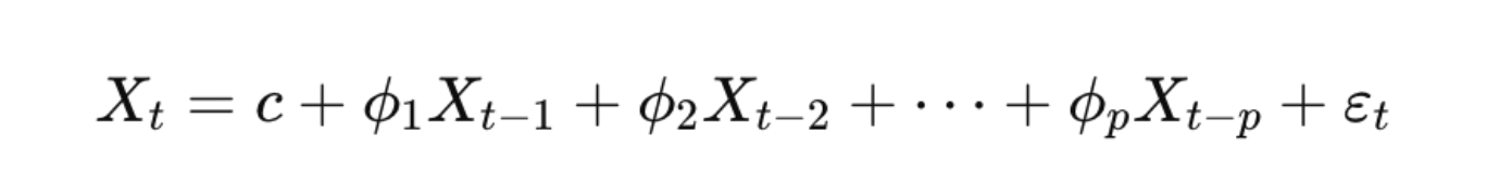
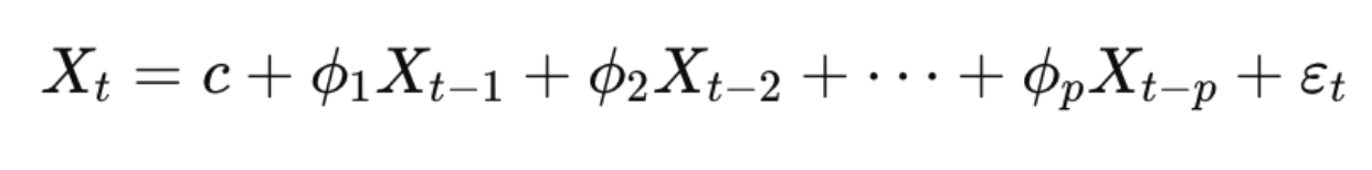
If we have to put this in the mathematical form, the general form of an Autoregressive model of order p, denoted as AR(p), is:
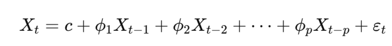
Where,
- Xt = value of the time series at time t
- c = constant term (intercept)
- ϕ1,ϕ2,…,ϕp = autoregressive coefficients (weights applied to past values)
- p = order of the model (number of lag terms)
- t = white noise error term (a random error with mean zero and constant variance)
This equation shows that if you want to predict Xtthe current value, which can be done by looking at a weighted sum of its p past values: Xt−1, Xt−2,…, Xt−p. The coefficients ϕ determine how much influence each lag has on the current value. The error term t accounts for randomness or influences not captured by the model.
Let us take an example of the AR(1) Model:
For an AR(1) model (autoregressive model of order 1), the equation becomes:
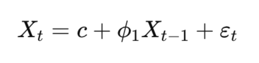
Here, each value is linearly dependent only on the immediately preceding value.
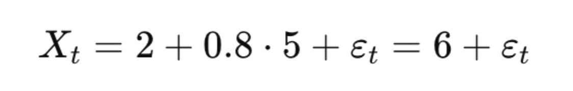
If:
- ϕ1=0.8
- c=2
- εt∼N
Then:
- If Xt−1=5, the expected value of Xt is:
One of the most important features of AR models is recursion:
Once a prediction is made for Xt, you can feed it back into the equation to predict Xt+1, and so on.
This is particularly useful for multi-step forecasting, where you’re predicting a sequence of future values based on the last known observation.
For an AR(p) model to be stable and reliable over time (i.e., stationary), the solutions to its characteristic equation must be greater than 1 in absolute value. In simple terms, this means the model’s behavior won’t keep growing or bouncing around wildly; it will settle around a consistent pattern.
For example, in AR(1):
∣ϕ1∣<1
This condition ensures that the influence of past values decays over time, and the series doesn’t explode or trend indefinitely.
Types of Autoregressive Models
Autoregressive models are categorized based on the number of lagged observations used to predict the current value of a time series. This number is referred to as the order of the model and is denoted by p in AR(p).
AR(1) – First Order Autoregressive Model
As we saw in our previous example, an AR(1) model uses just one lagged observation to predict the current value:
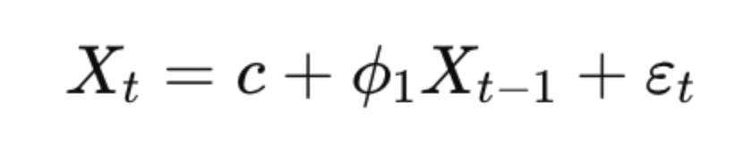
Here, Xt depends only on its immediate past value, Xt−1. It’s often used for modeling simple time series with short-term memory.
Common in financial time series or temperature data with short temporal dependencies.
AR(2) – Second Order Autoregressive Model
An AR(2) model uses two past values:
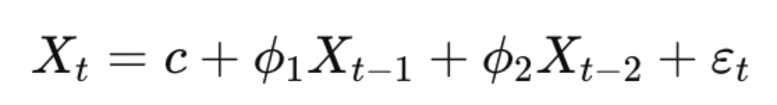
This model can capture more complex dynamics, such as cyclical behavior or delayed effects. The second lag allows the model to account for influence from two previous time steps.
AR(p) – General Autoregressive Model
In an AR(p) model, p lagged values are used:
Suitable for modeling time series with longer memory or more complex patterns. The choice of p is crucial; it determines how much past information is considered.
Choosing the Optimal Lag Value (p)
Selecting the right lag order p is essential for balancing model complexity and prediction accuracy. Too small a ppp may miss important patterns; too large a ppp may lead to overfitting.
Two commonly used criteria to select p are:
Akaike Information Criterion (AIC)
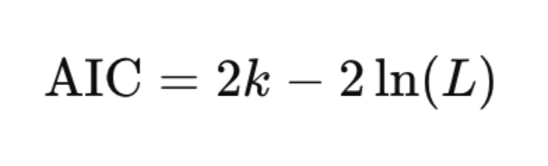
- k = number of parameters (including lag coefficients and intercept)
- L = maximized value of the likelihood function
- Lower AIC indicates a better model with a good tradeoff between fit and complexity.
- Prefers more complex models than BIC (more likely to avoid underfitting).
Bayesian Information Criterion (BIC)
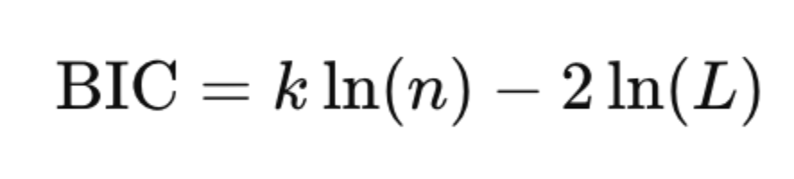
- n = number of observations
- Penalizes complexity more heavily than AIC.
- Better for smaller datasets or when you’re trying to avoid overfitting.
How to Build an AR Model (Step-by-Step)
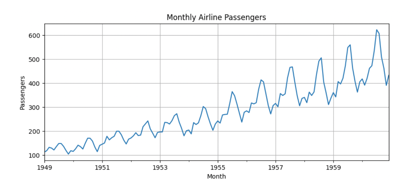
Step 1: Load and Visualize the Data
import pandas as pd
import matplotlib.pyplot as plt

# Load time series data (example: daily air passenger data)
url = 'https://raw.githubusercontent.com/jbrownlee/Datasets/master/airline-passengers.csv'
df = pd.read_csv(url, parse_dates=['Month'], index_col='Month')

# Rename column for convenience
df.rename(columns={'Passengers': 'Value'}, inplace=True)

# Plot the original time series
df['Value'].plot(figsize=(10, 4), title='Monthly Airline Passengers', ylabel='Passengers')
plt.grid(True)
plt.show()
Step 2: Check for Stationarity Using the ADF Test
Now, you might be wondering what is ADF test.
The Augmented Dickey-Fuller (ADF) test is a statistical test used to determine whether a time series is stationary or not.
A stationary time series is one whose mean, variance, and autocovariance are constant over time.
The ADF test checks for the presence of a unit root, which is a mathematical indication of non-stationarity.
ADF Test Hypotheses
The ADF test is a hypothesis test with the following setup:
- Null hypothesis (H₀): The time series has a unit root → the series is non-stationary
- Alternative hypothesis (H₁): The time series does not have a unit root → the series is stationary
So:
- If the p-value < 0.05 → reject the null → the series is stationary
- If the p-value ≥ 0.05 → fail to reject the null → the series is non-stationary
Now, in a stationary series, statistical patterns (like correlation with lags) are stable over time, making it easier to learn from the past. However, in non-stationary data, patterns can shift over time, which can lead to misleading results and poor forecasts.
If your time series is not stationary, you need to transform it (e.g., using differencing) before modeling.
from statsmodels.tsa.stattools import adfuller

# Augmented Dickey-Fuller test
result = adfuller(df['Value'])
print('ADF Statistic:', result[0])
print('p-value:', result[1])

if result[1] < 0.05:
    print("Series is stationary")
else:
    print("Series is NOT stationary")
ADF Statistic: 0.8153688792060498
p-value: 0.991880243437641
Series is NOT stationary
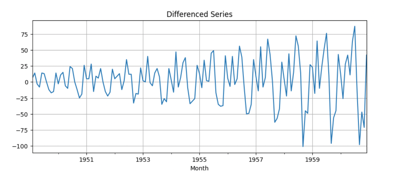
Step 3: Differencing to Achieve Stationarity
# First-order differencing
df_diff = df['Value'].diff().dropna()

# Recheck stationarity
result_diff = adfuller(df_diff)
print('ADF Statistic (Differenced):', result_diff[0])
print('p-value:', result_diff[1])

# Plot differenced series
df_diff.plot(figsize=(10, 4), title='Differenced Series')
plt.grid(True)
plt.show()
ADF Statistic (Differenced): -2.8292668241700047
p-value: 0.05421329028382478
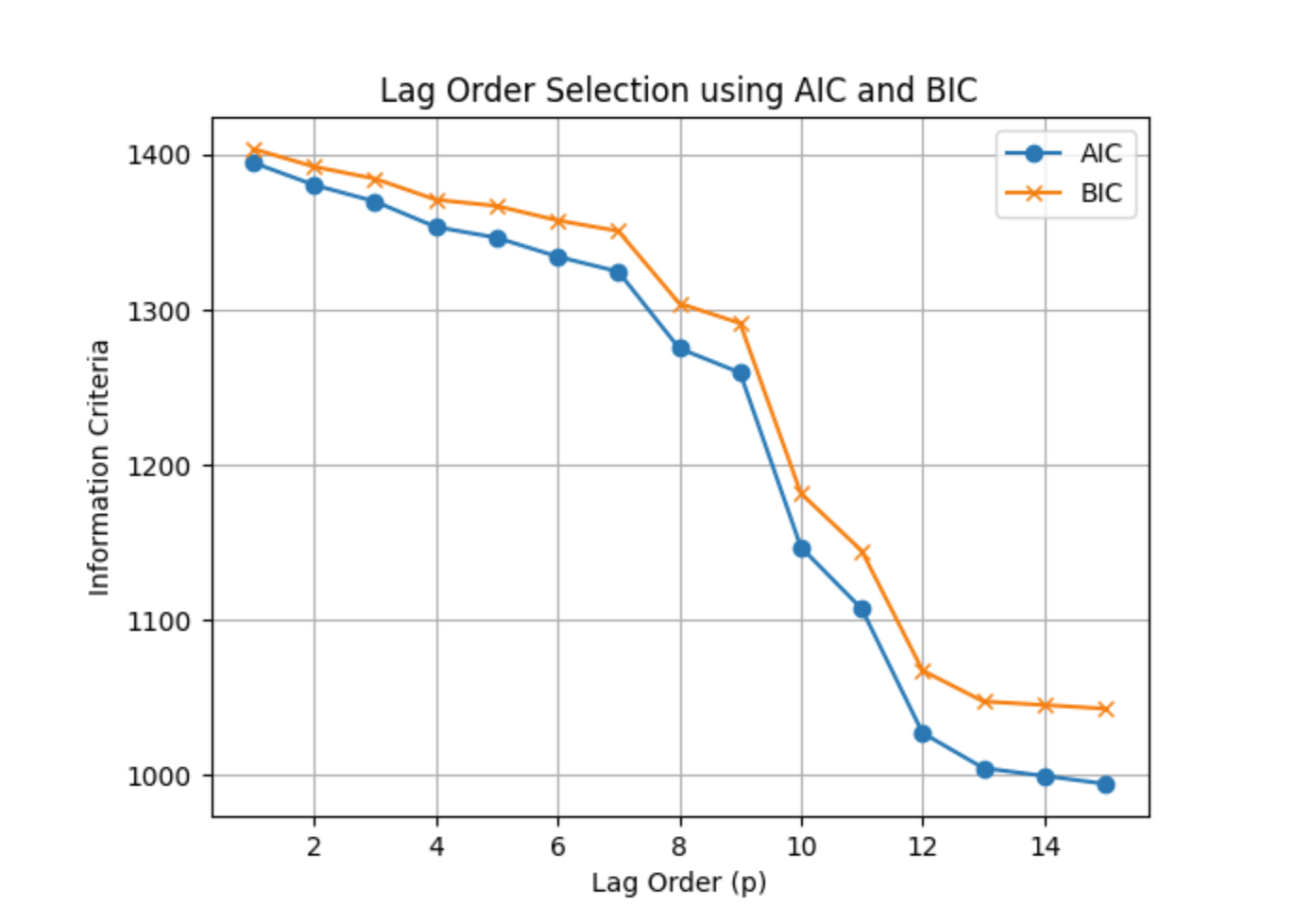
Step 4: Selecting Lag Order Using AIC/BIC
from statsmodels.tsa.ar_model import AutoReg

# Try models with lag 1 to 15 and compare AIC/BIC
aic_vals = []
bic_vals = []
lags = range(1, 16)

for p in lags:
    model = AutoReg(df_diff, lags=p, old_names=False).fit()
    aic_vals.append(model.aic)
    bic_vals.append(model.bic)

# Plot AIC and BIC scores
plt.plot(lags, aic_vals, label='AIC', marker='o')
plt.plot(lags, bic_vals, label='BIC', marker='x')
plt.xlabel('Lag Order (p)')
plt.ylabel('Information Criteria')
plt.title('Lag Order Selection using AIC and BIC')
plt.legend()
plt.grid(True)
plt.show()
Choose the lag p with the lowest AIC or BIC
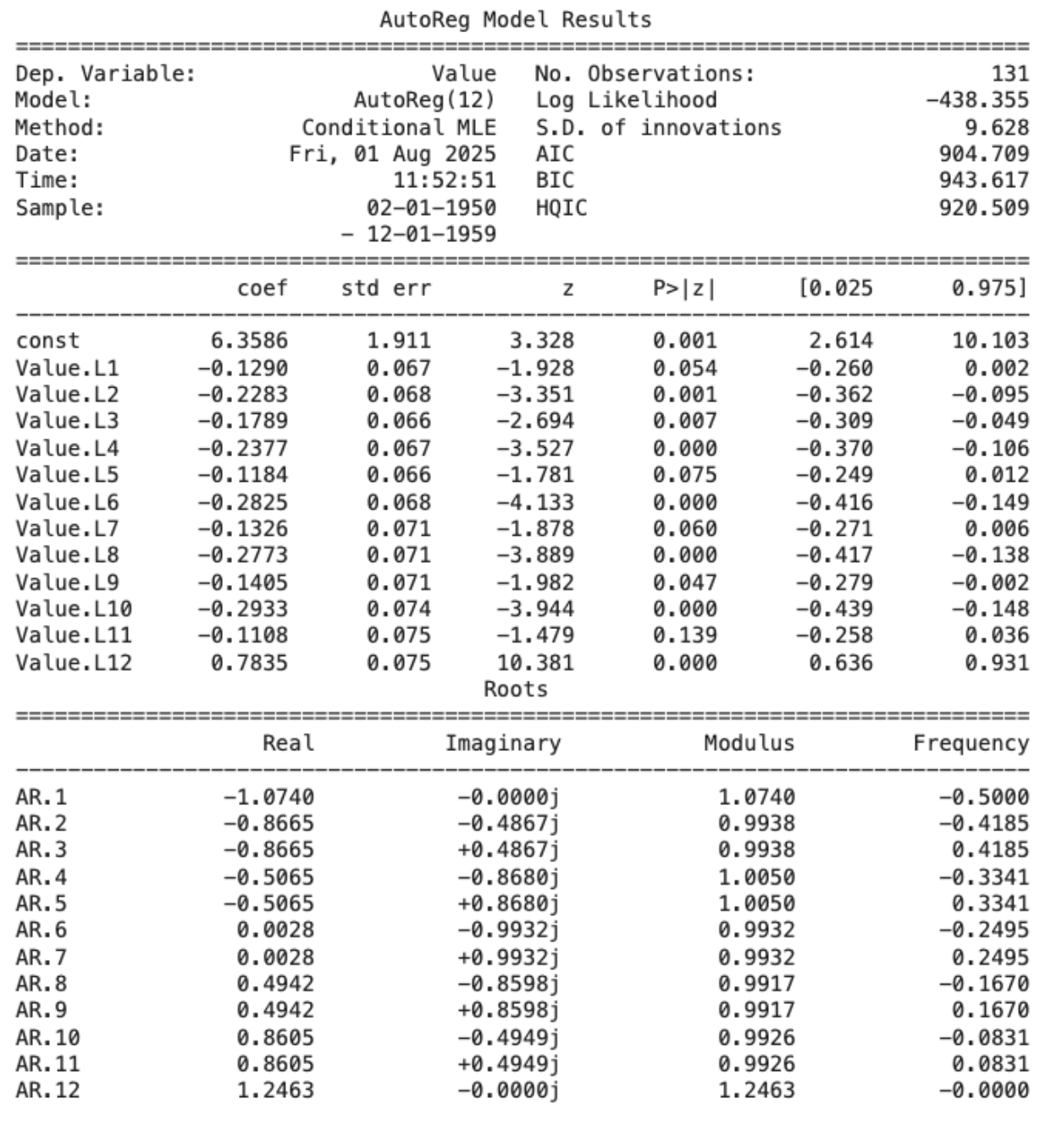
Step 5: Train the AR Model
# Choose optimal lag (e.g., p=4 from plot)
optimal_p = 4

# Split into train and test sets
train = df_diff[:-12]
test = df_diff[-12:]

# Fit the AR model
model = AutoReg(train, lags=optimal_p, old_names=False).fit()
print(model.summary())
Step 6: Make Predictions
# Predict the next 12 time steps
predictions = model.predict(start=len(train), end=len(train)+len(test)-1)

# Plot actual vs predicted
plt.figure(figsize=(10, 4))
plt.plot(test.index, test, label='Actual')
plt.plot(test.index, predictions, label='Predicted', linestyle='--')
plt.title('Actual vs Predicted (Differenced Series)')
plt.legend()
plt.grid(True)
plt.show()
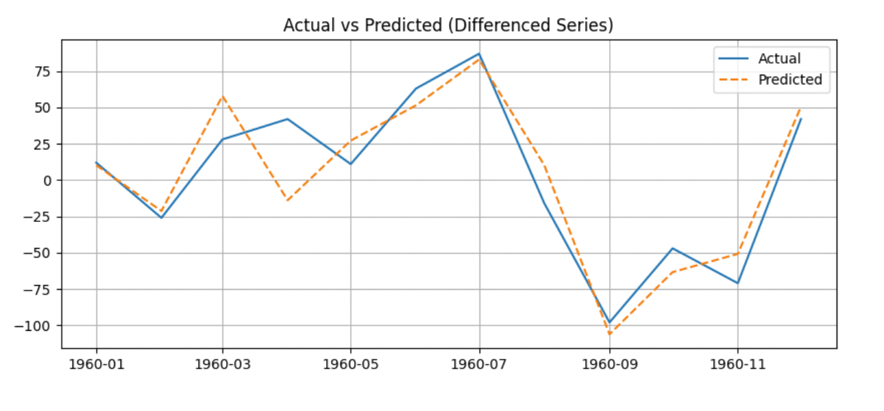
Step 7: Evaluate Performance (RMSE, MAE)
from sklearn.metrics import mean_squared_error, mean_absolute_error
import numpy as np

rmse = np.sqrt(mean_squared_error(test, predictions))
mae = mean_absolute_error(test, predictions)

print(f'RMSE: {rmse:.2f}')
print(f'MAE: {mae:.2f}')
RMSE: 22.28
MAE: 16.95
These values suggest that the AR model is performing well and can be trusted for short-term forecasting. However, it is best to check if the model is overfitting the data and to perform cross-validation techniques to verify the model’s accuracy.
Assumptions of AR Models
In order to build reliable and interpretable autoregressive models, there are certain statistical assumptions that must be satisfied. These assumptions are very necessary and if violated, can lead to inaccurate forecasts, unstable models, or misleading insights.
We already discussed Stationarity, which is one of the key assumptions. Here are a few other key assumptions that need to be considered:
Linearity
The AR model assumes a linear relationship between the current value and its past values (lags). That is:
Linear models are easier to interpret and solve. Non-linear relationships may not be captured well, which in turn leads to poor predictions.
To check the linearity, Plot actual vs predicted values and If the residuals show a pattern, consider using non-linear models (e.g., LSTM, non-linear AR).
No Autocorrelation in Residuals
After fitting the AR model, the residuals (errors) should be uncorrelated over time, i.e., they should look like random white noise.
If residuals are autocorrelated, it means the model missed some pattern that still exists in the data. This violates the assumption that all useful information is captured by the lags.
- Use Ljung-Box test or plot ACF of residuals.
- Further, residuals should not show significant spikes in autocorrelation plots.
Constant Variance (Homoscedasticity)
The variance of the residuals should remain constant over time. This is known as homoscedasticity. If the variance of residuals increases or decreases (i.e., heteroscedasticity), that shows the model’s error is not consistent. This can distort confidence intervals and make forecasts unreliable.
- Plot residuals over time and look for “funnel shapes” (increasing or decreasing spread).
- Use statistical tests like ARCH test for heteroscedasticity.
| Assumption | Description | Why It Matters | How to Check |
|---|---|---|---|
| Stationarity | Constant mean, variance, and autocorrelation over time | Ensures the model learns stable patterns | ADF test, plotting |
| Linearity | The current value is a linear function of past values | Core structure of AR models | Residual plots, visual inspection |
| No autocorrelation in errors | Residuals should behave like white noise | Indicates all patterns are captured | Ljung-Box test, ACF/PACF of residuals |
| Constant variance | Error variance should remain stable over time | Keeps forecast intervals valid | Residual plots, ARCH test |
AR vs. Other Time Series Models
Autoregressive (AR) models are a core building block in time series forecasting, but they’re not the only option. Here we will briefly discuss how the AR model differs from other time series.
AR vs. MA (Moving Average)
As we understood, AR (Autoregressive) uses past values of the series to predict future values. For example, today’s value depends on yesterday’s and the day before. However, MA (Moving Average) uses past errors (differences between actual and predicted values) to make predictions. It doesn’t directly use past values of the series.
Simple analogy:
Think of AR as saying, “Tomorrow will be like today,” while MA says, “Tomorrow will be adjusted based on how wrong we were yesterday.”
AR vs. ARMA and ARIMA
ARMA (Autoregressive Moving Average) combines both AR and MA models. It considers both past values and past errors.
ARIMA (Autoregressive Integrated Moving Average) adds a third component: differencing. It’s used when the data is non-stationary (i.e., its statistical properties like mean and variance change over time).
In short:
- Use AR when your data is stationary and has a strong relationship with its past values.
- Use ARMA if your stationary data also shows patterns in past errors.
- Use ARIMA if your data has trends or is not stationary. ARIMA first makes it stationary and then applies AR and MA.
Limitations of AR Models
While Autoregressive (AR) models are a great starting point for time series forecasting, they come with several limitations that are important to keep in mind. First, as we saw in this article, one of the AR models’ assumptions includes that the time series is stationary, meaning the mean, variance, and autocorrelation structure don’t change over time.
However, many real-world datasets like sales, weather patterns, or stock prices often have trends or seasonality, making them non-stationary and less suitable for AR without preprocessing. Additionally, AR models rely solely on past values of the time series to make predictions, which means they might perform poorly when external factors (like holidays, promotions, or unexpected events) significantly influence the data.
Another challenge is that AR models can become less accurate as the forecasting scope increases; the further out you try to predict, the more uncertain the predictions become, especially if the model order isn’t chosen carefully. Lastly, because AR models don’t account for errors from previous time steps (unlike MA or ARMA models), they might not handle random shocks or noise in the data as effectively. In short, while AR models are useful and interpretable, they work best under specific conditions and may need to be combined with other techniques for more complex forecasting tasks.
Frequently Asked Questions (FAQs)
Q1. What is an AR model used for in time series analysis?
An AR model is used to forecast future values based on past values in the same time series. It’s especially useful when data shows strong temporal dependencies and remains statistically stable over time.
Q2. When should I not use an AR model?
Avoid using AR when your data is non-stationary, has strong seasonal trends, or is heavily influenced by external variables. In such cases, models like ARIMA or SARIMA are more appropriate.
Q3. What’s the difference between AR and ARIMA?
AR uses only past values for prediction, while ARIMA adds differencing to handle trends and a moving average (MA) component to account for past errors, making it better for non-stationary data.
Q4. How do I know if my time series data is stationary?
You can use statistical tests like the Augmented Dickey-Fuller (ADF) test or visualize the data to check for constant mean and variance over time. If not, differencing may be needed to make it stationary.
Q5. Can AR models be used for multivariate time series?
Basic AR models are univariate. For multivariate forecasting, you’d look into extensions like Vector Autoregression (VAR), which captures relationships across multiple time-dependent variables.
Conclusion
Understanding the AR model can be a beginner-friendly foundational technique in time series forecasting. One of AR model’s core strengths lies in its simplicity and interpretability. An AR model makes future predictions by learning patterns from past values of the same series. This makes AR models particularly useful when you’re dealing with stationary data and want to model straightforward dependencies over time. AR serves as the building block for more advanced models. It helps lay the groundwork for understanding how past behavior can inform future trends, which is a key idea in time series analysis. However, as we move toward more real-world applications, data often becomes messier, with trends, seasonality, and external influences. This is where the AR model starts to show its limitations.
Its Role in the Bigger Picture
- AR is ideal for basic, stationary time series where the primary driver of future values is the past itself.
- It provides a baseline model against which more complex models can be evaluated.
- It is a key component in more comprehensive models like ARMA and ARIMA, acting as the “AR” part of those hybrids.
Once you’re comfortable with AR, there are several directions to explore:
- ARIMA (Autoregressive Integrated Moving Average): Useful when your data shows trends or is non-stationary. ARIMA introduces differencing and adds a moving average component to model residuals better.
- SARIMA (Seasonal ARIMA): Extends ARIMA to handle seasonal patterns, which are common in monthly or quarterly data.
- LSTM (Long Short-Term Memory networks): A deep learning-based model that can capture long-range dependencies, nonlinear trends, and complex patterns. Ideal for large datasets with intricate time-based behavior.
Each of these models builds on the foundation that AR provides, offering more flexibility and power for handling the complexities of real-world time series data.
Useful Resources
- https://medium.com/@phylypo/overview-of-time-series-forecasting-from-statistical-to-recent-ml-approaches-c51a5dd4656a
- https://www.kaggle.com/code/prashant111/complete-guide-on-time-series-analysis-in-python
- https://www.kaggle.com/code/satishgunjal/tutorial-time-series-analysis-and-forecasting
- https://www.digitalocean.com/community/tutorials/a-guide-to-time-series-visualization-with-python-3
- https://www.digitalocean.com/community/tutorials/a-guide-to-time-series-forecasting-with-arima-in-python-3
- https://www.digitalocean.com/community/tutorials/a-guide-to-time-series-visualization-with-python-3
Thanks for learning with the DigitalOcean Community. Check out our offerings for compute, storage, networking, and managed databases.
About the author
With a strong background in data science and over six years of experience, I am passionate about creating in-depth content on technologies. Currently focused on AI, machine learning, and GPU computing, working on topics ranging from deep learning frameworks to optimizing GPU-based workloads.
Still looking for an answer?
This textbox defaults to using Markdown to format your answer.
You can type !ref in this text area to quickly search our full set of tutorials, documentation & marketplace offerings and insert the link!
 This work is licensed under a Creative Commons Attribution-NonCommercial- ShareAlike 4.0 International License.
Become a contributor for community
Get paid to write technical tutorials and select a tech-focused charity to receive a matching donation.

DigitalOcean Documentation
Full documentation for every DigitalOcean product.

Resources for startups and AI-native businesses
The Wave has everything you need to know about building a business, from raising funding to marketing your product.
The developer cloud
Scale up as you grow — whether you're running one virtual machine or ten thousand.

Start building today
From GPU-powered inference and Kubernetes to managed databases and storage, get everything you need to build, scale, and deploy intelligent applications.
