By Alvin Wan and Brian Hogan

The author selected Girls Who Code to receive a donation as part of the Write for DOnations program.
Introduction
Computer vision is a subfield of computer science that aims to extract a higher-order understanding from images and videos. This field includes tasks such as object detection, image restoration (matrix completion), and optical flow. Computer vision powers technologies such as self-driving car prototypes, employee-less grocery stores, fun Snapchat filters, and your mobile device’s face authenticator.
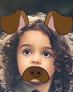
In this tutorial, you will explore computer vision as you use pre-trained models to build a Snapchat-esque dog filter. For those unfamiliar with Snapchat, this filter will detect your face and then superimpose a dog mask on it. You will then train a face-emotion classifier so that the filter can pick dog masks based on emotion, such as a corgi for happy or a pug for sad. Along the way, you will also explore related concepts in both ordinary least squares and computer vision, which will expose you to the fundamentals of machine learning.
As you work through the tutorial, you’ll use OpenCV, a computer-vision library, numpy for linear algebra utilities, and matplotlib for plotting. You’ll also apply the following concepts as you build a computer-vision application:
- Ordinary least squares as a regression and classification technique.
- The basics of stochastic gradient neural networks.
While not necessary to complete this tutorial, you’ll find it easier to understand some of the more detailed explanations if you’re familiar with these mathematical concepts:
- Fundamental linear algebra concepts: scalars, vectors, and matrices.
- Fundamental calculus: how to take a derivative.
You can find the complete code for this tutorial at https://github.com/do-community/emotion-based-dog-filter.
Let’s get started.
Prerequisites
To complete this tutorial, you will need the following:
- A local development environment for Python 3 with at least 1GB of RAM. You can follow How To Install and Set Up a Local Programming Environment for Python 3 to configure everything you need.
- A working webcam to do real-time image detection.
Step 1 — Creating The Project and Installing Dependencies
Let’s create a workspace for this project and install the dependencies we’ll need. We’ll call our workspace DogFilter:
- mkdir ~/DogFilter
Navigate to the DogFilter directory:
- cd ~/DogFilter
Then create a new Python virtual environment for the project:
- python3 -m venv dogfilter
Activate your environment.
- source dogfilter/bin/activate
The prompt changes, indicating the environment is active. Now install PyTorch, a deep-learning framework for Python that we’ll use in this tutorial. The installation process depends on which operating system you’re using.
On macOS, install Pytorch with the following command:
- python -m pip install torch==0.4.1 torchvision==0.2.1
On Linux, use the following commands:
- pip install http://download.pytorch.org/whl/cpu/torch-0.4.1-cp35-cp35m-linux_x86_64.whl
- pip install torchvision
And for Windows, install Pytorch with these commands:
- pip install http://download.pytorch.org/whl/cpu/torch-0.4.1-cp35-cp35m-win_amd64.whl
- pip install torchvision
Now install prepackaged binaries for OpenCV and numpy, which are computer vision and linear algebra libraries, respectively. The former offers utilities such as image rotations, and the latter offers linear algebra utilities such as a matrix inversion.
- python -m pip install opencv-python==3.4.3.18 numpy==1.14.5
Finally, create a directory for our assets, which will hold the images we’ll use in this tutorial:
- mkdir assets
With the dependencies installed, let’s build the first version of our filter: a face detector.
Step 2 — Building a Face Detector
Our first objective is to detect all faces in an image. We’ll create a script that accepts a single image and outputs an annotated image with the faces outlined with boxes.
Fortunately, instead of writing our own face detection logic, we can use pre-trained models. We’ll set up a model and then load pre-trained parameters. OpenCV makes this easy by providing both.
OpenCV provides the model parameters in its source code. but we need the absolute path to our locally-installed OpenCV to use these parameters. Since that absolute path may vary, we’ll download our own copy instead and place it in the assets folder:
- wget -O assets/haarcascade_frontalface_default.xml https://github.com/opencv/opencv/raw/master/data/haarcascades/haarcascade_frontalface_default.xml
The -O option specifies the destination as assets/haarcascade_frontalface_default.xml. The second argument is the source URL.
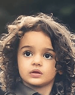
We’ll detect all faces in the following image from Pexels (CC0, link to original image).

First, download the image. The following command saves the downloaded image as children.png in the assets folder:
- wget -O assets/children.png https://assets.digitalocean.com/articles/python3_dogfilter/CfoBWbF.png
To check that the detection algorithm works, we will run it on an individual image and save the resulting annotated image to disk. Create an outputs folder for these annotated results.
- mkdir outputs
Now create a Python script for the face detector. Create the file step_1_face_detect using nano or your favorite text editor:
- nano step_2_face_detect.py
Add the following code to the file. This code imports OpenCV, which contains the image utilities and face classifier. The rest of the code is typical Python program boilerplate.
"""Test for face detection"""

import cv2


def main():
    pass

if __name__ == '__main__':
    main()
Now replace pass in the main function with this code which initializes a face classifier using the OpenCV parameters you downloaded to your assets folder:
def main():
    # initialize front face classifier
    cascade = cv2.CascadeClassifier("assets/haarcascade_frontalface_default.xml")
Next, add this line to load the image children.png.
frame = cv2.imread('assets/children.png')
Then add this code to convert the image to black and white, as the classifier was trained on black-and-white images. To accomplish this, we convert to grayscale and then discretize the histogram:
    # Convert to black-and-white
    gray = cv2.cvtColor(frame, cv2.COLOR_BGR2GRAY)
    blackwhite = cv2.equalizeHist(gray)
Then use OpenCV’s detectMultiScale function to detect all faces in the image.
    rects = cascade.detectMultiScale(
        blackwhite, scaleFactor=1.3, minNeighbors=4, minSize=(30, 30),
        flags=cv2.CASCADE_SCALE_IMAGE)
scaleFactorspecifies how much the image is reduced along each dimension.minNeighborsdenotes how many neighboring rectangles a candidate rectangle needs to be retained.minSizeis the minimum allowable detected object size. Objects smaller than this are discarded.
The return type is a list of tuples, where each tuple has four numbers denoting the minimum x, minimum y, width, and height of the rectangle in that order.
Iterate over all detected objects and draw them on the image in green using cv2.rectangle:
    for x, y, w, h in rects:
        cv2.rectangle(frame, (x, y), (x + w, y + h), (0, 255, 0), 2)
- The second and third arguments are opposing corners of the rectangle.
- The fourth argument is the color to use.
(0, 255, 0)corresponds to green for our RGB color space. - The last argument denotes the width of our line.
Finally, write the image with bounding boxes into a new file at outputs/children_detected.png:
cv2.imwrite('outputs/children_detected.png', frame)
Your completed script should look like this:
"""Tests face detection for a static image."""

import cv2


def main():

    # initialize front face classifier
    cascade = cv2.CascadeClassifier(
        "assets/haarcascade_frontalface_default.xml")

    frame = cv2.imread('assets/children.png')

    # Convert to black-and-white
    gray = cv2.cvtColor(frame, cv2.COLOR_BGR2GRAY)
    blackwhite = cv2.equalizeHist(gray)

    rects = cascade.detectMultiScale(
        blackwhite, scaleFactor=1.3, minNeighbors=4, minSize=(30, 30),
    flags=cv2.CASCADE_SCALE_IMAGE)

    for x, y, w, h in rects:
        cv2.rectangle(frame, (x, y), (x + w, y + h), (0, 255, 0), 2)

    cv2.imwrite('outputs/children_detected.png', frame)

if __name__ == '__main__':
    main()
Save the file and exit your editor. Then run the script:
- python step_2_face_detect.py
Open outputs/children_detected.png. You’ll see the following image that shows the faces outlined with boxes:
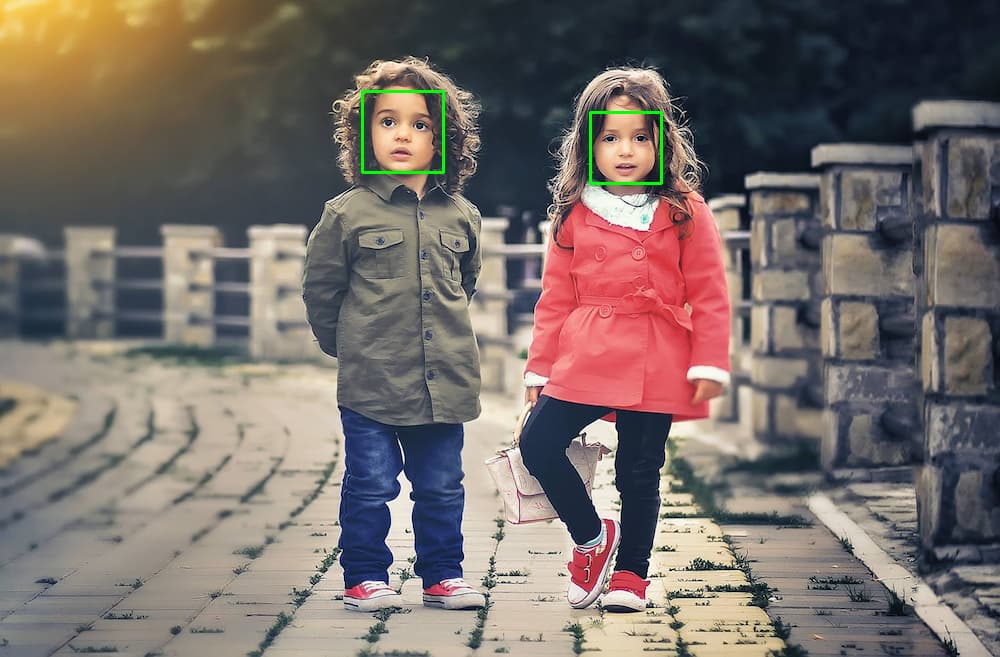
At this point, you have a working face detector. It accepts an image as input and draws bounding boxes around all faces in the image, outputting the annotated image. Now let’s apply this same detection to a live camera feed.
Step 3 — Linking the Camera Feed
The next objective is to link the computer’s camera to the face detector. Instead of detecting faces in a static image, you’ll detect all faces from your computer’s camera. You will collect camera input, detect and annotate all faces, and then display the annotated image back to the user. You’ll continue from the script in Step 2, so start by duplicating that script:
- cp step_2_face_detect.py step_3_camera_face_detect.py
Then open the new script in your editor:
- nano step_3_camera_face_detect.py
You will update the main function by using some elements from this test script from the official OpenCV documentation. Start by initializing a VideoCapture object that is set to capture live feed from your computer’s camera. Place this at the start of the main function, before the other code in the function:
def main():
    cap = cv2.VideoCapture(0)
    ...
Starting from the line defining frame, indent all of your existing code, placing all of the code in a while loop.
    while True:
        frame = cv2.imread('assets/children.png')
        ...
        for x, y, w, h in rects:
            cv2.rectangle(frame, (x, y), (x + w, y + h), (0, 255, 0), 2)

        cv2.imwrite('outputs/children_detected.png', frame)
Replace the line defining frame at the start of the while loop. Instead of reading from an image on disk, you’re now reading from the camera:
    while True:
        # frame = cv2.imread('assets/children.png') # DELETE ME
        # Capture frame-by-frame
        ret, frame = cap.read()
Replace the line cv2.imwrite(...) at the end of the while loop. Instead of writing an image to disk, you’ll display the annotated image back to the user’s screen:
      cv2.imwrite('outputs/children_detected.png', frame)  # DELETE ME
      # Display the resulting frame
      cv2.imshow('frame', frame)
Also, add some code to watch for keyboard input so you can stop the program. Check if the user hits the q character and, if so, quit the application. Right after cv2.imshow(...) add the following:
...
        cv2.imshow('frame', frame)
        if cv2.waitKey(1) & 0xFF == ord('q'):
            break
...
The line cv2.waitkey(1) halts the program for 1 millisecond so that the captured image can be displayed back to the user.
Finally, release the capture and close all windows. Place this outside of the while loop to end the main function.
...

    while True:
    ...


    cap.release()
    cv2.destroyAllWindows()
Your script should look like the following:
"""Test for face detection on video camera.

Move your face around and a green box will identify your face.
With the test frame in focus, hit `q` to exit.
Note that typing `q` into your terminal will do nothing.
"""

import cv2


def main():
    cap = cv2.VideoCapture(0)

    # initialize front face classifier
    cascade = cv2.CascadeClassifier(
        "assets/haarcascade_frontalface_default.xml")

    while True:
        # Capture frame-by-frame
        ret, frame = cap.read()

        # Convert to black-and-white
        gray = cv2.cvtColor(frame, cv2.COLOR_BGR2GRAY)
        blackwhite = cv2.equalizeHist(gray)

        # Detect faces
        rects = cascade.detectMultiScale(
            blackwhite, scaleFactor=1.3, minNeighbors=4, minSize=(30, 30),
            flags=cv2.CASCADE_SCALE_IMAGE)

        # Add all bounding boxes to the image
        for x, y, w, h in rects:
            cv2.rectangle(frame, (x, y), (x + w, y + h), (0, 255, 0), 2)

        # Display the resulting frame
        cv2.imshow('frame', frame)
        if cv2.waitKey(1) & 0xFF == ord('q'):
            break

    # When everything done, release the capture
    cap.release()
    cv2.destroyAllWindows()


if __name__ == '__main__':
    main()
Save the file and exit your editor.
Now run the test script.
- python step_3_camera_face_detect.py
This activates your camera and opens a window displaying your camera’s feed. Your face will be boxed by a green square in real time:
Note: If you find that you have to hold very still for things to work, the lighting in the room may not be adequate. Try moving to a brightly lit room where you and your background have high constrast. Also, avoid bright lights near your head. For example, if you have your back to the sun, this process might not work very well.
Our next objective is to take the detected faces and superimpose dog masks on each one.
Step 4 — Building the Dog Filter
Before we build the filter itself, let’s explore how images are represented numerically. This will give you the background needed to modify images and ultimately apply a dog filter.
Let’s look at an example. We can construct a black-and-white image using numbers, where 0 corresponds to black and 1 corresponds to white.
Focus on the dividing line between 1s and 0s. What shape do you see?
0 0 0 0 0 0 0 0 0
0 0 0 0 1 0 0 0 0
0 0 0 1 1 1 0 0 0
0 0 1 1 1 1 1 0 0
0 0 0 1 1 1 0 0 0
0 0 0 0 1 0 0 0 0
0 0 0 0 0 0 0 0 0
The image is a diamond. If save this matrix of values as an image. This gives us the following picture:

We can use any value between 0 and 1, such as 0.1, 0.26, or 0.74391. Numbers closer to 0 are darker and numbers closer to 1 are lighter. This allows us to represent white, black, and any shade of gray. This is great news for us because we can now construct any grayscale image using 0, 1, and any value in between. Consider the following, for example. Can you tell what it is? Again, each number corresponds to the color of a pixel.
1  1  1  1  1  1  1  1  1  1  1  1
1  1  1  1  0  0  0  0  1  1  1  1
1  1  0  0 .4 .4 .4 .4  0  0  1  1
1  0 .4 .4 .5 .4 .4 .4 .4 .4  0  1
1  0 .4 .5 .5 .5 .4 .4 .4 .4  0  1
0 .4 .4 .4 .5 .4 .4 .4 .4 .4 .4  0
0 .4 .4 .4 .4  0  0 .4 .4 .4 .4  0
0  0 .4 .4  0  1 .7  0 .4 .4  0  0
0  1  0  0  0 .7 .7  0  0  0  1  0
1  0  1  1  1  0  0 .7 .7 .4  0  1
1  0 .7  1  1  1 .7 .7 .7 .7  0  1
1  1  0  0 .7 .7 .7 .7  0  0  1  1
1  1  1  1  0  0  0  0  1  1  1  1
1  1  1  1  1  1  1  1  1  1  1  1
Re-rendered as an image, you can now tell that this is, in fact, a Poké Ball:

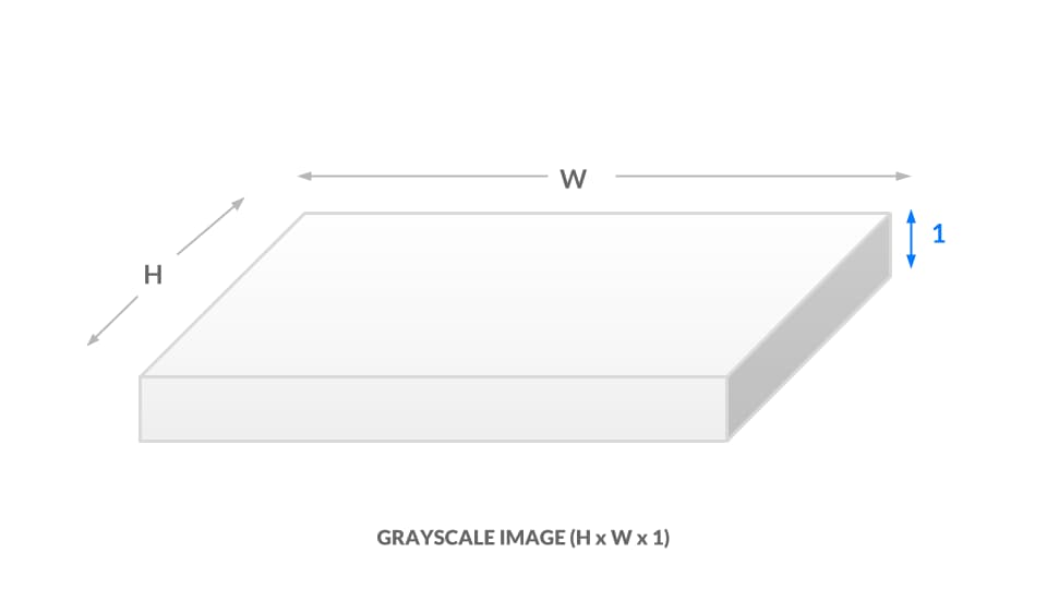
You’ve now seen how black-and-white and grayscale images are represented numerically. To introduce color, we need a way to encode more information. An image has its height and width expressed as h x w.
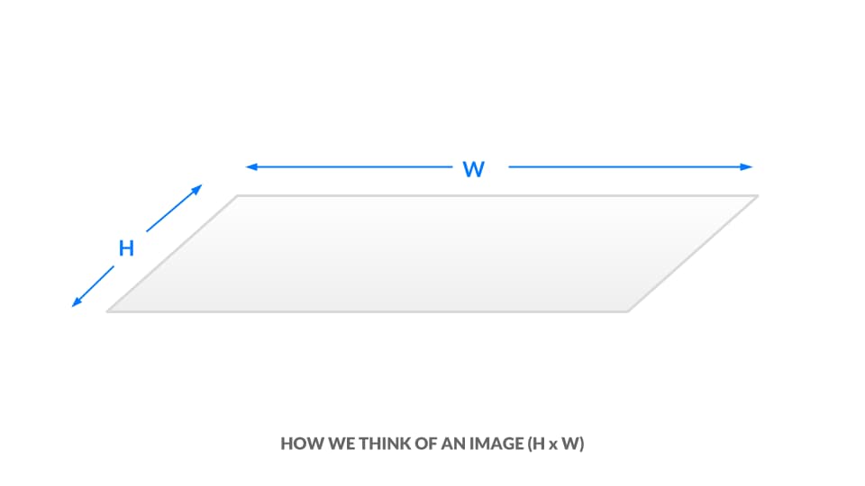
In the current grayscale representation, each pixel is one value between 0 and 1. We can equivalently say our image has dimensions h x w x 1. In other words, every (x, y) position in our image has just one value.
For a color representation, we represent the color of each pixel using three values between 0 and 1. One number corresponds to the “degree of red,” one to the “degree of green,” and the last to the “degree of blue.” We call this the RGB color space. This means that for every (x, y) position in our image, we have three values (r, g, b). As a result, our image is now h x w x 3:
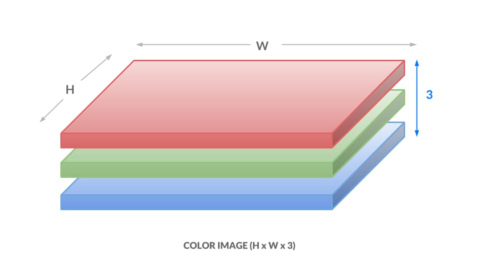
Here, each number ranges from 0 to 255 instead of 0 to 1, but the idea is the same. Different combinations of numbers correspond to different colors, such as dark purple (102, 0, 204) or bright orange (255, 153, 51). The takeaways are as follows:
- Each image will be represented as a box of numbers that has three dimensions: height, width, and color channels. Manipulating this box of numbers directly is equivalent to manipulating the image.
- We can also flatten this box to become just a list of numbers. In this way, our image becomes a vector. Later on, we will refer to images as vectors.
Now that you understand how images are represented numerically, you are well-equipped to begin applying dog masks to faces. To apply a dog mask, you will replace values in the child image with non-white dog mask pixels. To start, you will work with a single image. Download this crop of a face from the image you used in Step 2.
- wget -O assets/child.png https://assets.digitalocean.com/articles/python3_dogfilter/alXjNK1.png
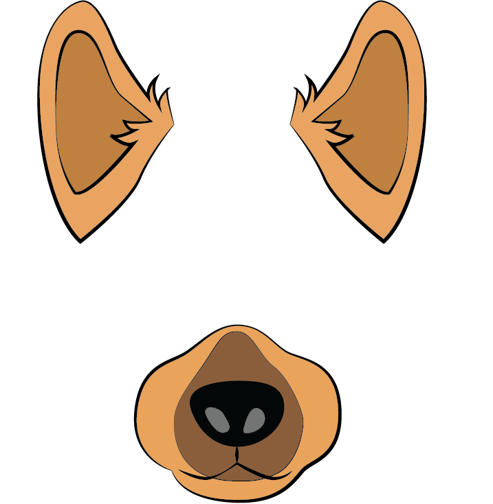
Additionally, download the following dog mask. The dog masks used in this tutorial are my own drawings, now released to the public domain under a CC0 License.
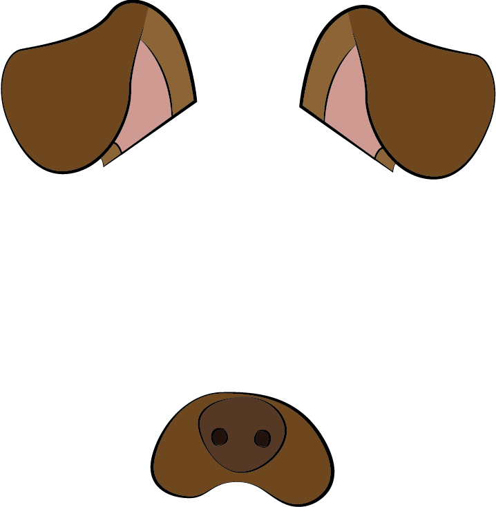
Download this with wget:
- wget -O assets/dog.png https://assets.digitalocean.com/articles/python3_dogfilter/ED32BCs.png
Create a new file called step_4_dog_mask_simple.py which will hold the code for the script that applies the dog mask to faces:
- nano step_4_dog_mask_simple.py
Add the following boilerplate for the Python script and import the OpenCV and numpy libraries:
"""Test for adding dog mask"""

import cv2
import numpy as np


def main():
    pass

if __name__ == '__main__':
    main()
Replace pass in the main function with these two lines which load the original image and the dog mask into memory.
...
def main():
    face = cv2.imread('assets/child.png')
    mask = cv2.imread('assets/dog.png')
Next, fit the dog mask to the child. The logic is more complicated than what we’ve done previously, so we will create a new function called apply_mask to modularize our code. Directly after the two lines that load the images, add this line which invokes the apply_mask function:
...
    face_with_mask = apply_mask(face, mask)
Create a new function called apply_mask and place it above the main function:
...
def apply_mask(face: np.array, mask: np.array) -> np.array:
    """Add the mask to the provided face, and return the face with mask."""
    pass

def main():
...
At this point, your file should look like this:
"""Test for adding dog mask"""

import cv2
import numpy as np


def apply_mask(face: np.array, mask: np.array) -> np.array:
    """Add the mask to the provided face, and return the face with mask."""
    pass


def main():
    face = cv2.imread('assets/child.png')
    mask = cv2.imread('assets/dog.png')
    face_with_mask = apply_mask(face, mask)

if __name__ == '__main__':
    main()
Let’s build out the apply_mask function. Our goal is to apply the mask to the child’s face. However, we need to maintain the aspect ratio for our dog mask. To do so, we need to explicitly compute our dog mask’s final dimensions. Inside the apply_mask function, replace pass with these two lines which extract the height and width of both images:
...
    mask_h, mask_w, _ = mask.shape
    face_h, face_w, _ = face.shape
Next, determine which dimension needs to be “shrunk more.” To be precise, we need the tighter of the two constraints. Add this line to the apply_mask function:
...

    # Resize the mask to fit on face
    factor = min(face_h / mask_h, face_w / mask_w)
Then compute the new shape by adding this code to the function:
...
    new_mask_w = int(factor * mask_w)
    new_mask_h = int(factor * mask_h)
    new_mask_shape = (new_mask_w, new_mask_h)
Here we cast the numbers to integers, as the resize function needs integral dimensions.
Now add this code to resize the dog mask to the new shape:
...

    # Add mask to face - ensure mask is centered
    resized_mask = cv2.resize(mask, new_mask_shape)
Finally, write the image to disk so you can double-check that your resized dog mask is correct after you run the script:
cv2.imwrite('outputs/resized_dog.png', resized_mask)
The completed script should look like this:
"""Test for adding dog mask"""
import cv2
import numpy as np

def apply_mask(face: np.array, mask: np.array) -> np.array:
    """Add the mask to the provided face, and return the face with mask."""
    mask_h, mask_w, _ = mask.shape
    face_h, face_w, _ = face.shape

    # Resize the mask to fit on face
    factor = min(face_h / mask_h, face_w / mask_w)
    new_mask_w = int(factor * mask_w)
    new_mask_h = int(factor * mask_h)
    new_mask_shape = (new_mask_w, new_mask_h)

    # Add mask to face - ensure mask is centered
    resized_mask = cv2.resize(mask, new_mask_shape)
    cv2.imwrite('outputs/resized_dog.png', resized_mask)


def main():
    face = cv2.imread('assets/child.png')
    mask = cv2.imread('assets/dog.png')
    face_with_mask = apply_mask(face, mask)

if __name__ == '__main__':
    main()
Save the file and exit your editor. Run the new script:
- python step_4_dog_mask_simple.py
Open the image at outputs/resized_dog.png to double-check the mask was resized correctly. It will match the dog mask shown earlier in this section.
Now add the dog mask to the child. Open the step_4_dog_mask_simple.py file again and return to the apply_mask function:
- nano step_4_dog_mask_simple.py
First, remove the line of code that writes the resized mask from the apply_mask function since you no longer need it:
    cv2.imwrite('outputs/resized_dog.png', resized_mask)  # delete this line
    ...
In its place, apply your knowledge of image representation from the start of this section to modify the image. Start by making a copy of the child image. Add this line to the apply_mask function:
...
    face_with_mask = face.copy()
Next, find all positions where the dog mask is not white or near white. To do this, check if the pixel value is less than 250 across all color channels, as we’d expect a near-white pixel to be near [255, 255, 255]. Add this code:
...
    non_white_pixels = (resized_mask < 250).all(axis=2)
At this point, the dog image is, at most, as large as the child image. We want to center the dog image on the face, so compute the offset needed to center the dog image by adding this code to apply_mask:
...
    off_h = int((face_h - new_mask_h) / 2)
    off_w = int((face_w - new_mask_w) / 2)
Copy all non-white pixels from the dog image into the child image. Since the child image may be larger than the dog image, we need to take a subset of the child image:
    face_with_mask[off_h: off_h+new_mask_h, off_w: off_w+new_mask_w][non_white_pixels] = \
            resized_mask[non_white_pixels]
Then return the result:
return face_with_mask
In the main function, add this code to write the result of the apply_mask function to an output image so you can manually double-check the result:
...
    face_with_mask = apply_mask(face, mask)
    cv2.imwrite('outputs/child_with_dog_mask.png', face_with_mask)
Your completed script will look like the following:
"""Test for adding dog mask"""

import cv2
import numpy as np


def apply_mask(face: np.array, mask: np.array) -> np.array:
    """Add the mask to the provided face, and return the face with mask."""
    mask_h, mask_w, _ = mask.shape
    face_h, face_w, _ = face.shape

    # Resize the mask to fit on face
    factor = min(face_h / mask_h, face_w / mask_w)
    new_mask_w = int(factor * mask_w)
    new_mask_h = int(factor * mask_h)
    new_mask_shape = (new_mask_w, new_mask_h)
    resized_mask = cv2.resize(mask, new_mask_shape)

    # Add mask to face - ensure mask is centered
    face_with_mask = face.copy()
    non_white_pixels = (resized_mask < 250).all(axis=2)
    off_h = int((face_h - new_mask_h) / 2)
    off_w = int((face_w - new_mask_w) / 2)
    face_with_mask[off_h: off_h+new_mask_h, off_w: off_w+new_mask_w][non_white_pixels] = \
         resized_mask[non_white_pixels]

    return face_with_mask

def main():
    face = cv2.imread('assets/child.png')
    mask = cv2.imread('assets/dog.png')
    face_with_mask = apply_mask(face, mask)
    cv2.imwrite('outputs/child_with_dog_mask.png', face_with_mask)

if __name__ == '__main__':
    main()
Save the script and run it:
- python step_4_dog_mask_simple.py
You’ll have the following picture of a child with a dog mask in outputs/child_with_dog_mask.png:
You now have a utility that applies dog masks to faces. Now let’s use what you’ve built to add the dog mask in real time.
We’ll pick up from where we left off in Step 3. Copy step_3_camera_face_detect.py to step_4_dog_mask.py.
- cp step_3_camera_face_detect.py step_4_dog_mask.py
Open your new script.
- nano step_4_dog_mask.py
First, import the NumPy library at the top of the script:
import numpy as np
...
Then add the apply_mask function from your previous work into this new file above the main function:
def apply_mask(face: np.array, mask: np.array) -> np.array:
    """Add the mask to the provided face, and return the face with mask."""
    mask_h, mask_w, _ = mask.shape
    face_h, face_w, _ = face.shape

    # Resize the mask to fit on face
    factor = min(face_h / mask_h, face_w / mask_w)
    new_mask_w = int(factor * mask_w)
    new_mask_h = int(factor * mask_h)
    new_mask_shape = (new_mask_w, new_mask_h)
    resized_mask = cv2.resize(mask, new_mask_shape)

    # Add mask to face - ensure mask is centered
    face_with_mask = face.copy()
    non_white_pixels = (resized_mask < 250).all(axis=2)
    off_h = int((face_h - new_mask_h) / 2)
    off_w = int((face_w - new_mask_w) / 2)
    face_with_mask[off_h: off_h+new_mask_h, off_w: off_w+new_mask_w][non_white_pixels] = \
         resized_mask[non_white_pixels]

    return face_with_mask
...
Second, locate this line in the main function:
cap = cv2.VideoCapture(0)
Add this code after that line to load the dog mask:
    cap = cv2.VideoCapture(0)

    # load mask
    mask = cv2.imread('assets/dog.png')
    ...
Next, in the while loop, locate this line:
ret, frame = cap.read()
Add this line after it to extract the image’s height and width:
        ret, frame = cap.read()
        frame_h, frame_w, _ = frame.shape
        ...
Next, delete the line in main that draws bounding boxes. You’ll find this line in the for loop that iterates over detected faces:
        for x, y, w, h in rects:
        ...
            cv2.rectangle(frame, (x, y), (x + w, y + h), (0, 255, 0), 2) # DELETE ME
        ...
In its place, add this code which crops the frame. For aesthetic purposes, we crop an area slightly larger than the face.
        for x, y, w, h in rects:
            # crop a frame slightly larger than the face
            y0, y1 = int(y - 0.25*h), int(y + 0.75*h)
            x0, x1 = x, x + w
Introduce a check in case the detected face is too close to the edge.
            # give up if the cropped frame would be out-of-bounds
            if x0 < 0 or y0 < 0 or x1 > frame_w or y1 > frame_h:
                continue
Finally, insert the face with a mask into the image.
            # apply mask
            frame[y0: y1, x0: x1] = apply_mask(frame[y0: y1, x0: x1], mask)
Verify that your script looks like this:
"""Real-time dog filter

Move your face around and a dog filter will be applied to your face if it is not out-of-bounds. With the test frame in focus, hit `q` to exit. Note that typing `q` into your terminal will do nothing.
"""

import numpy as np
import cv2


def apply_mask(face: np.array, mask: np.array) -> np.array:
    """Add the mask to the provided face, and return the face with mask."""
    mask_h, mask_w, _ = mask.shape
    face_h, face_w, _ = face.shape

    # Resize the mask to fit on face
    factor = min(face_h / mask_h, face_w / mask_w)
    new_mask_w = int(factor * mask_w)
    new_mask_h = int(factor * mask_h)
    new_mask_shape = (new_mask_w, new_mask_h)
    resized_mask = cv2.resize(mask, new_mask_shape)

    # Add mask to face - ensure mask is centered
    face_with_mask = face.copy()
    non_white_pixels = (resized_mask < 250).all(axis=2)
    off_h = int((face_h - new_mask_h) / 2)
    off_w = int((face_w - new_mask_w) / 2)
    face_with_mask[off_h: off_h+new_mask_h, off_w: off_w+new_mask_w][non_white_pixels] = \
         resized_mask[non_white_pixels]

    return face_with_mask

def main():
    cap = cv2.VideoCapture(0)

    # load mask
    mask = cv2.imread('assets/dog.png')

    # initialize front face classifier
    cascade = cv2.CascadeClassifier("assets/haarcascade_frontalface_default.xml")

    while(True):
        # Capture frame-by-frame
        ret, frame = cap.read()
        frame_h, frame_w, _ = frame.shape

        # Convert to black-and-white
        gray = cv2.cvtColor(frame, cv2.COLOR_BGR2GRAY)
        blackwhite = cv2.equalizeHist(gray)

        # Detect faces
        rects = cascade.detectMultiScale(
            blackwhite, scaleFactor=1.3, minNeighbors=4, minSize=(30, 30),
            flags=cv2.CASCADE_SCALE_IMAGE)

        # Add mask to faces
        for x, y, w, h in rects:
            # crop a frame slightly larger than the face
            y0, y1 = int(y - 0.25*h), int(y + 0.75*h)
            x0, x1 = x, x + w

            # give up if the cropped frame would be out-of-bounds
            if x0 < 0 or y0 < 0 or x1 > frame_w or y1 > frame_h:
                continue

            # apply mask
            frame[y0: y1, x0: x1] = apply_mask(frame[y0: y1, x0: x1], mask)

        # Display the resulting frame
        cv2.imshow('frame', frame)
        if cv2.waitKey(1) & 0xFF == ord('q'):
            break

    # When everything done, release the capture
    cap.release()
    cv2.destroyAllWindows()


if __name__ == '__main__':
    main()
Save the file and exit your editor. Then run the script.
- python step_4_dog_mask.py
You now have a real-time dog filter running. The script will also work with multiple faces in the picture, so you can get your friends together for some automatic dog-ification.
This concludes our first primary objective in this tutorial, which is to create a Snapchat-esque dog filter. Now let’s use facial expression to determine the dog mask applied to a face.
Step 5 — Build a Basic Face Emotion Classifier using Least Squares
In this section you’ll create an emotion classifier to apply different masks based on displayed emotions. If you smile, the filter will apply a corgi mask. If you frown, it will apply a pug mask. Along the way, you’ll explore the least-squares framework, which is fundamental to understanding and discussing machine learning concepts.
To understand how to process our data and produce predictions, we’ll first briefly explore machine learning models.
We need to ask two questions for each model that we consider. For now, these two questions will be sufficient to differentiate between models:
- Input: What information is the model given?
- Output: What is the model trying to predict?
At a high-level, the goal is to develop a model for emotion classification. The model is:
- Input: given images of faces.
- Output: predicts the corresponding emotion.
model: face -> emotion
The approach we’ll use is least squares; we take a set of points, and we find a line of best fit. The line of best fit, shown in the following image, is our model.
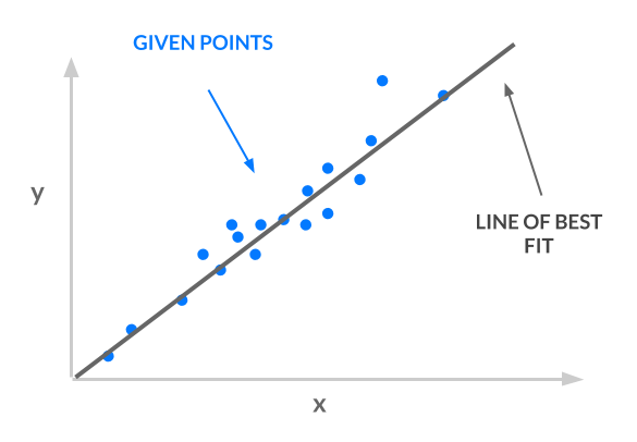
Consider the input and output for our line:
- Input: given
xcoordinates. - Output: predicts the corresponding $y$ coordinate.
least squares line: x -> y
Our input x must represent faces and our output y must represent emotion, in order for us to use least squares for emotion classification:
x -> face: Instead of using one number forx, we will use a vector of values forx. Thus,xcan represent images of faces. The article Ordinary Least Squares explains why you can use a vector of values forx.y -> emotion: Each emotion will correspond to a number. For example, “angry” is 0, “sad” is 1, and “happy” is 2. In this way,ycan represent emotions. However, our line is not constrained to output theyvalues 0, 1, and 2. It has an infinite number of possible y values–it could be 1.2, 3.5, or 10003.42. How do we translate thoseyvalues to integers corresponding to classes? See the article One-Hot Encoding for more detail and explanation.
Armed with this background knowledge, you will build a simple least-squares classifier using vectorized images and one-hot encoded labels. You’ll accomplish this in three steps:
- Preprocess the data: As explained at the start of this section, our samples are vectors where each vector encodes an image of a face. Our labels are integers corresponding to an emotion, and we’ll apply one-hot encoding to these labels.
- Specify and train the model: Use the closed-form least squares solution,
w^*. - Run a prediction using the model: Take the argmax of
Xw^*to obtain predicted emotions.
Let’s get started.
First, set up a directory to contain the data:
- mkdir data
Then download the data, curated by Pierre-Luc Carrier and Aaron Courville, from a 2013 Face Emotion Classification competition on Kaggle.
- wget -O data/fer2013.tar https://bitbucket.org/alvinwan/adversarial-examples-in-computer-vision-building-then-fooling/raw/babfe4651f89a398c4b3fdbdd6d7a697c5104cff/fer2013.tar
Navigate to the data directory and unpack the data.
- cd data
- tar -xzf fer2013.tar
Now we’ll create a script to run the least-squares model. Navigate to the root of your project:
- cd ~/DogFilter
Create a new file for the script:
- nano step_5_ls_simple.py
Add Python boilerplate and import the packages you will need:
"""Train emotion classifier using least squares."""

import numpy as np

def main():
    pass

if __name__ == '__main__':
    main()
Next, load the data into memory. Replace pass in your main function with the following code:
    # load data
    with np.load('data/fer2013_train.npz') as data:
        X_train, Y_train = data['X'], data['Y']

    with np.load('data/fer2013_test.npz') as data:
        X_test, Y_test = data['X'], data['Y']
Now one-hot encode the labels. To do this, construct the identity matrix with numpy and then index into this matrix using our list of labels:
    # one-hot labels
    I = np.eye(6)
    Y_oh_train, Y_oh_test = I[Y_train], I[Y_test]
Here, we use the fact that the i-th row in the identity matrix is all zero, except for the i-th entry. Thus, the i-th row is the one-hot encoding for the label of class i. Additionally, we use numpy’s advanced indexing, where [a, b, c, d][[1, 3]] = [b, d].
Computing (X^TX)^{-1} would take too long on commodity hardware, as X^TX is a 2304x2304 matrix with over four million values, so we’ll reduce this time by selecting only the first 100 features. Add this code:
...
    # select first 100 dimensions
    A_train, A_test = X_train[:, :100], X_test[:, :100]
Next, add this code to evaluate the closed-form least-squares solution:
...
    # train model
    w = np.linalg.inv(A_train.T.dot(A_train)).dot(A_train.T.dot(Y_oh_train))
Then define an evaluation function for training and validation sets. Place this before your main function:
def evaluate(A, Y, w):
    Yhat = np.argmax(A.dot(w), axis=1)
    return np.sum(Yhat == Y) / Y.shape[0]
To estimate labels, we take the inner product with each sample and get the indices of the maximum values using np.argmax. Then we compute the average number of correct classifications. This final number is your accuracy.
Finally, add this code to the end of the main function to compute the training and validation accuracy using the evaluate function you just wrote:
    # evaluate model
    ols_train_accuracy = evaluate(A_train, Y_train, w)
    print('(ols) Train Accuracy:', ols_train_accuracy)
    ols_test_accuracy = evaluate(A_test, Y_test, w)
    print('(ols) Test Accuracy:', ols_test_accuracy)
Double-check that your script matches the following:
"""Train emotion classifier using least squares."""

import numpy as np


def evaluate(A, Y, w):
    Yhat = np.argmax(A.dot(w), axis=1)
    return np.sum(Yhat == Y) / Y.shape[0]

def main():

    # load data
    with np.load('data/fer2013_train.npz') as data:
        X_train, Y_train = data['X'], data['Y']

    with np.load('data/fer2013_test.npz') as data:
        X_test, Y_test = data['X'], data['Y']

    # one-hot labels
    I = np.eye(6)
    Y_oh_train, Y_oh_test = I[Y_train], I[Y_test]

    # select first 100 dimensions
    A_train, A_test = X_train[:, :100], X_test[:, :100]

    # train model
    w = np.linalg.inv(A_train.T.dot(A_train)).dot(A_train.T.dot(Y_oh_train))

    # evaluate model
    ols_train_accuracy = evaluate(A_train, Y_train, w)
    print('(ols) Train Accuracy:', ols_train_accuracy)
    ols_test_accuracy = evaluate(A_test, Y_test, w)
    print('(ols) Test Accuracy:', ols_test_accuracy)


if __name__ == '__main__':
    main()
Save your file, exit your editor, and run the Python script.
- python step_5_ls_simple.py
You’ll see the following output:
Output(ols) Train Accuracy: 0.4748918316507146
(ols) Test Accuracy: 0.45280545359202934
Our model gives 47.5% train accuracy. We repeat this on the validation set to obtain 45.3% accuracy. For a three-way classification problem, 45.3% is reasonably above guessing, which is 33%. This is our starting classifier for emotion detection, and in the next step, you’ll build off of this least-squares model to improve accuracy. The higher the accuracy, the more reliably your emotion-based dog filter can find the appropriate dog filter for each detected emotion.
Step 6 — Improving Accuracy by Featurizing the Inputs
We can use a more expressive model to boost accuracy. To accomplish this, we featurize our inputs.
The original image tells us that position (0, 0) is red, (1, 0) is brown, and so on. A featurized image may tell us that there is a dog to the top-left of the image, a person in the middle, etc. Featurization is powerful, but its precise definition is beyond the scope of this tutorial.
We’ll use an approximation for the radial basis function (RBF) kernel, using a random Gaussian matrix. We won’t go into detail in this tutorial. Instead, we’ll treat this as a black box that computes higher-order features for us.
We’ll continue where we left off in the previous step. Copy the previous script so you have a good starting point:
- cp step_5_ls_simple.py step_6_ls_simple.py
Open the new file in your editor:
- nano step_6_ls_simple.py
We’ll start by creating the featurizing random matrix. Again, we’ll use only 100 features in our new feature space.
Locate the following line, defining A_train and A_test:
    # select first 100 dimensions
    A_train, A_test = X_train[:, :100], X_test[:, :100]
Directly above this definition for A_train and A_test, add a random feature matrix:
    d = 100
    W = np.random.normal(size=(X_train.shape[1], d))
    # select first 100 dimensions
    A_train, A_test = X_train[:, :100], X_test[:, :100]  ...
Then replace the definitions for A_train and A_test. We redefine our matrices, called design matrices, using this random featurization.
A_train, A_test = X_train.dot(W), X_test.dot(W)
Save your file and run the script.
- python step_6_ls_simple.py
You’ll see the following output:
Output(ols) Train Accuracy: 0.584174642717
(ols) Test Accuracy: 0.584425799685
This featurization now offers 58.4% train accuracy and 58.4% validation accuracy, a 13.1% improvement in validation results. We trimmed the X matrix to be 100 x 100, but the choice of 100 was arbirtary. We could also trim the X matrix to be 1000 x 1000 or 50 x 50. Say the dimension of x is d x d. We can test more values of d by re-trimming X to be d x d and recomputing a new model.
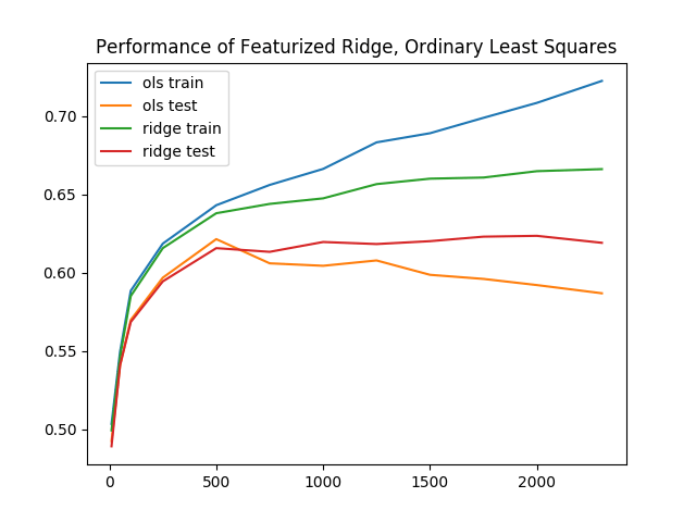
Trying more values of d, we find an additional 4.3% improvement in test accuracy to 61.7%. In the following figure, we consider the performance of our new classifier as we vary d. Intuitively, as d increases, the accuracy should also increase, as we use more and more of our original data. Rather than paint a rosy picture, however, the graph exhibits a negative trend:
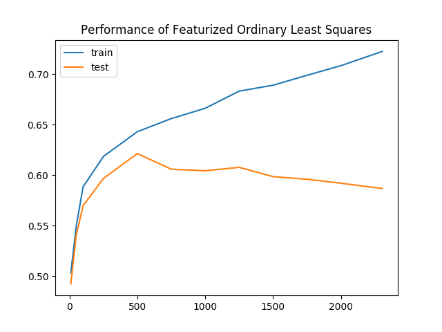
As we keep more of our data, the gap between the training and validation accuracies increases as well. This is clear evidence of overfitting, where our model is learning representations that are no longer generalizable to all data. To combat overfitting, we’ll regularize our model by penalizing complex models.
We amend our ordinary least-squares objective function with a regularization term, giving us a new objective. Our new objective function is called ridge regression and it looks like this:
min_w |Aw- y|^2 + lambda |w|^2
In this equation, lambda is a tunable hyperparameter. Plug lambda = 0 into the equation and ridge regression becomes least-squares. Plug lambda = infinity into the equation, and you’ll find the best w must now be zero, as any non-zero w incurs infinite loss. As it turns out, this objective yields a closed-form solution as well:
w^* = (A^TA + lambda I)^{-1}A^Ty
Still using the featurized samples, retrain and reevaluate the model once more.
Open step_6_ls_simple.py again in your editor:
- nano step_6_ls_simple.py
This time, increase the dimensionality of the new feature space to d=1000. Change the value of d from 100 to 1000 as shown in the following code block:
...
    d = 1000
    W = np.random.normal(size=(X_train.shape[1], d))
...
Then apply ridge regression using a regularization of lambda = 10^{10}. Replace the line defining w with the following two lines:
...
    # train model
    I = np.eye(A_train.shape[1])
    w = np.linalg.inv(A_train.T.dot(A_train) + 1e10 * I).dot(A_train.T.dot(Y_oh_train))
Then locate this block:
...
  ols_train_accuracy = evaluate(A_train, Y_train, w)
  print('(ols) Train Accuracy:', ols_train_accuracy)
  ols_test_accuracy = evaluate(A_test, Y_test, w)
  print('(ols) Test Accuracy:', ols_test_accuracy)
Replace it with the following:
...

  print('(ridge) Train Accuracy:', evaluate(A_train, Y_train, w))
  print('(ridge) Test Accuracy:', evaluate(A_test, Y_test, w))
The completed script should look like this:
"""Train emotion classifier using least squares."""

import numpy as np

def evaluate(A, Y, w):
    Yhat = np.argmax(A.dot(w), axis=1)
    return np.sum(Yhat == Y) / Y.shape[0]

def main():
    # load data
    with np.load('data/fer2013_train.npz') as data:
        X_train, Y_train = data['X'], data['Y']

    with np.load('data/fer2013_test.npz') as data:
        X_test, Y_test = data['X'], data['Y']

    # one-hot labels
    I = np.eye(6)
    Y_oh_train, Y_oh_test = I[Y_train], I[Y_test]
    d = 1000
    W = np.random.normal(size=(X_train.shape[1], d))
    # select first 100 dimensions
    A_train, A_test = X_train.dot(W), X_test.dot(W)

    # train model
    I = np.eye(A_train.shape[1])
    w = np.linalg.inv(A_train.T.dot(A_train) + 1e10 * I).dot(A_train.T.dot(Y_oh_train))

    # evaluate model
    print('(ridge) Train Accuracy:', evaluate(A_train, Y_train, w))
    print('(ridge) Test Accuracy:', evaluate(A_test, Y_test, w))

if __name__ == '__main__':
    main()
Save the file, exit your editor, and run the script:
- python step_6_ls_simple.py
You’ll see the following output:
Output(ridge) Train Accuracy: 0.651173462698
(ridge) Test Accuracy: 0.622181436812
There’s an additional improvement of 0.4% in validation accuracy to 62.2%, as train accuracy drops to 65.1%. Once again reevaluating across a number of different d, we see a smaller gap between training and validation accuracies for ridge regression. In other words, ridge regression was subject to less overfitting.
Baseline performance for least squares, with these extra enhancements, performs reasonably well. The training and inference times, all together, take no more than 20 seconds for even the best results. In the next section, you’ll explore even more complex models.
Step 7 — Building the Face-Emotion Classifier Using a Convolutional Neural Network in PyTorch
In this section, you’ll build a second emotion classifier using neural networks instead of least squares. Again, our goal is to produce a model that accepts faces as input and outputs an emotion. Eventually, this classifier will then determine which dog mask to apply.
For a brief neural network visualization and introduction, see the article Understanding Neural Networks. Here, we will use a deep-learning library called PyTorch. There are a number of deep-learning libraries in widespread use, and each has various pros and cons. PyTorch is a particularly good place to start. To impliment this neural network classifier, we again take three steps, as we did with the least-squares classifier:
- Preprocess the data: Apply one-hot encoding and then apply PyTorch abstractions.
- Specify and train the model: Set up a neural network using PyTorch layers. Define optimization hyperparameters and run stochastic gradient descent.
- Run a prediction using the model: Evaluate the neural network.
Create a new file, named step_7_fer_simple.py
- nano step_7_fer_simple.py
Import the necessary utilities and create a Python class that will hold your data. For data processing here, you will create the train and test datasets. To do these, implement PyTorch’s Dataset interface, which lets you load and use PyTorch’s built-in data pipeline for the face-emotion recognition dataset:
from torch.utils.data import Dataset
from torch.autograd import Variable
import torch.nn as nn
import torch.nn.functional as F
import torch.optim as optim
import numpy as np
import torch
import cv2
import argparse


class Fer2013Dataset(Dataset):
    """Face Emotion Recognition dataset.

    Utility for loading FER into PyTorch. Dataset curated by Pierre-Luc Carrier
    and Aaron Courville in 2013.

    Each sample is 1 x 1 x 48 x 48, and each label is a scalar.
    """
    pass
Delete the pass placeholder in the Fer2013Dataset class. In its place, add a function that will initialize our data holder:
    def __init__(self, path: str):
        """
        Args:
            path: Path to `.np` file containing sample nxd and label nx1
        """
        with np.load(path) as data:
            self._samples = data['X']
            self._labels = data['Y']
        self._samples = self._samples.reshape((-1, 1, 48, 48))

        self.X = Variable(torch.from_numpy(self._samples)).float()
        self.Y = Variable(torch.from_numpy(self._labels)).float()
...
This function starts by loading the samples and labels. Then it wraps the data in PyTorch data structures.
Directly after the __init__ function, add a __len__ function, as this is needed to implement the Dataset interface PyTorch expects:
...
    def __len__(self):
        return len(self._labels)
Finally, add a __getitem__ method, which returns a dictionary containing the sample and the label:
    def __getitem__(self, idx):
        return {'image': self._samples[idx], 'label': self._labels[idx]}
Double-check that your file looks like the following:
from torch.utils.data import Dataset
from torch.autograd import Variable
import torch.nn as nn
import torch.nn.functional as F
import torch.optim as optim
import numpy as np
import torch
import cv2
import argparse


class Fer2013Dataset(Dataset):
    """Face Emotion Recognition dataset.
    Utility for loading FER into PyTorch. Dataset curated by Pierre-Luc Carrier
    and Aaron Courville in 2013.
    Each sample is 1 x 1 x 48 x 48, and each label is a scalar.
    """

    def __init__(self, path: str):
        """
        Args:
            path: Path to `.np` file containing sample nxd and label nx1
        """
        with np.load(path) as data:
            self._samples = data['X']
            self._labels = data['Y']
        self._samples = self._samples.reshape((-1, 1, 48, 48))

        self.X = Variable(torch.from_numpy(self._samples)).float()
        self.Y = Variable(torch.from_numpy(self._labels)).float()

    def __len__(self):
        return len(self._labels)

    def __getitem__(self, idx):
        return {'image': self._samples[idx], 'label': self._labels[idx]}
Next, load the Fer2013Dataset dataset. Add the following code to the end of your file after the Fer2013Dataset class:
trainset = Fer2013Dataset('data/fer2013_train.npz')
trainloader = torch.utils.data.DataLoader(trainset, batch_size=32, shuffle=True)

testset = Fer2013Dataset('data/fer2013_test.npz')
testloader = torch.utils.data.DataLoader(testset, batch_size=32, shuffle=False)
This code initializes the dataset using the Fer2013Dataset class you created. Then for the train and validation sets, it wraps the dataset in a DataLoader. This translates the dataset into an iterable to use later.
As a sanity check, verify that the dataset utilities are functioning. Create a sample dataset loader using DataLoader and print the first element of that loader. Add the following to the end of your file:
if __name__ == '__main__':
    loader = torch.utils.data.DataLoader(trainset, batch_size=2, shuffle=False)
    print(next(iter(loader)))
Verify that your completed script looks like this:
from torch.utils.data import Dataset
from torch.autograd import Variable
import torch.nn as nn
import torch.nn.functional as F
import torch.optim as optim
import numpy as np
import torch
import cv2
import argparse


class Fer2013Dataset(Dataset):
    """Face Emotion Recognition dataset.
    Utility for loading FER into PyTorch. Dataset curated by Pierre-Luc Carrier
    and Aaron Courville in 2013.
    Each sample is 1 x 1 x 48 x 48, and each label is a scalar.
    """

    def __init__(self, path: str):
        """
        Args:
            path: Path to `.np` file containing sample nxd and label nx1
        """
        with np.load(path) as data:
            self._samples = data['X']
            self._labels = data['Y']
        self._samples = self._samples.reshape((-1, 1, 48, 48))

        self.X = Variable(torch.from_numpy(self._samples)).float()
        self.Y = Variable(torch.from_numpy(self._labels)).float()

    def __len__(self):
        return len(self._labels)

    def __getitem__(self, idx):
        return {'image': self._samples[idx], 'label': self._labels[idx]}

trainset = Fer2013Dataset('data/fer2013_train.npz')
trainloader = torch.utils.data.DataLoader(trainset, batch_size=32, shuffle=True)

testset = Fer2013Dataset('data/fer2013_test.npz')
testloader = torch.utils.data.DataLoader(testset, batch_size=32, shuffle=False)

if __name__ == '__main__':
    loader = torch.utils.data.DataLoader(trainset, batch_size=2, shuffle=False)
    print(next(iter(loader)))
Exit your editor and run the script.
- python step_7_fer_simple.py
This outputs the following pair of tensors. Our data pipeline outputs two samples and two labels. This indicates that our data pipeline is up and ready to go:
Output{'image':
(0 ,0 ,.,.) =
   24   32   36  ...   173  172  173
   25   34   29  ...   173  172  173
   26   29   25  ...   172  172  174
      ...         ⋱        ...
  159  185  157  ...   157  156  153
  136  157  187  ...   152  152  150
  145  130  161  ...   142  143  142
     ⋮

(1 ,0 ,.,.) =
   20   17   19  ...   187  176  162
   22   17   17  ...   195  180  171
   17   17   18  ...   203  193  175
      ...         ⋱        ...
    1    1    1  ...   106  115  119
    2    2    1  ...   103  111  119
    2    2    2  ...    99  107  118
[torch.LongTensor of size 2x1x48x48]
, 'label':
 1
 1
[torch.LongTensor of size 2]
}
Now that you’ve verified that the data pipeline works, return to step_7_fer_simple.py to add the neural network and optimizer. Open step_7_fer_simple.py.
- nano step_7_fer_simple.py
First, delete the last three lines you added in the previous iteration:
# Delete all three lines
if __name__ == '__main__':
    loader = torch.utils.data.DataLoader(trainset, batch_size=2, shuffle=False)
    print(next(iter(loader)))
In their place, define a PyTorch neural network that includes three convolutional layers, followed by three fully connected layers. Add this to the end of your existing script:
class Net(nn.Module):
    def __init__(self):
        super(Net, self).__init__()
        self.conv1 = nn.Conv2d(1, 6, 5)
        self.pool = nn.MaxPool2d(2, 2)
        self.conv2 = nn.Conv2d(6, 6, 3)
        self.conv3 = nn.Conv2d(6, 16, 3)
        self.fc1 = nn.Linear(16 * 4 * 4, 120)
        self.fc2 = nn.Linear(120, 48)
        self.fc3 = nn.Linear(48, 3)

    def forward(self, x):
        x = self.pool(F.relu(self.conv1(x)))
        x = self.pool(F.relu(self.conv2(x)))
        x = self.pool(F.relu(self.conv3(x)))
        x = x.view(-1, 16 * 4 * 4)
        x = F.relu(self.fc1(x))
        x = F.relu(self.fc2(x))
        x = self.fc3(x)
        return x
Now initialize the neural network, define a loss function, and define optimization hyperparameters by adding the following code to the end of the script:
net = Net().float()
criterion = nn.CrossEntropyLoss()
optimizer = optim.SGD(net.parameters(), lr=0.001, momentum=0.9)
We’ll train for two epochs. For now, we define an epoch to be an iteration of training where every training sample has been used exactly once.
First, extract image and label from the dataset loader and then wrap each in a PyTorch Variable. Second, run the forward pass and then backpropagate through the loss and neural network. Add the following code to the end of your script to do that:
for epoch in range(2):  # loop over the dataset multiple times

    running_loss = 0.0
    for i, data in enumerate(trainloader, 0):
        inputs = Variable(data['image'].float())
        labels = Variable(data['label'].long())
        optimizer.zero_grad()

        # forward + backward + optimize
        outputs = net(inputs)
        loss = criterion(outputs, labels)
        loss.backward()
        optimizer.step()

        # print statistics
        running_loss += loss.data[0]
        if i % 100 == 0:
            print('[%d, %5d] loss: %.3f' % (epoch, i, running_loss / (i + 1)))
Your script should now look like this:
from torch.utils.data import Dataset
from torch.autograd import Variable
import torch.nn as nn
import torch.nn.functional as F
import torch.optim as optim
import numpy as np
import torch
import cv2
import argparse


class Fer2013Dataset(Dataset):
    """Face Emotion Recognition dataset.

    Utility for loading FER into PyTorch. Dataset curated by Pierre-Luc Carrier
    and Aaron Courville in 2013.

    Each sample is 1 x 1 x 48 x 48, and each label is a scalar.
    """
    def __init__(self, path: str):
        """
        Args:
            path: Path to `.np` file containing sample nxd and label nx1
        """
        with np.load(path) as data:
            self._samples = data['X']
            self._labels = data['Y']
        self._samples = self._samples.reshape((-1, 1, 48, 48))

        self.X = Variable(torch.from_numpy(self._samples)).float()
        self.Y = Variable(torch.from_numpy(self._labels)).float()

    def __len__(self):
        return len(self._labels)


    def __getitem__(self, idx):
        return {'image': self._samples[idx], 'label': self._labels[idx]}


trainset = Fer2013Dataset('data/fer2013_train.npz')
trainloader = torch.utils.data.DataLoader(trainset, batch_size=32, shuffle=True)

testset = Fer2013Dataset('data/fer2013_test.npz')
testloader = torch.utils.data.DataLoader(testset, batch_size=32, shuffle=False)


class Net(nn.Module):
    def __init__(self):
        super(Net, self).__init__()
        self.conv1 = nn.Conv2d(1, 6, 5)
        self.pool = nn.MaxPool2d(2, 2)
        self.conv2 = nn.Conv2d(6, 6, 3)
        self.conv3 = nn.Conv2d(6, 16, 3)
        self.fc1 = nn.Linear(16 * 4 * 4, 120)
        self.fc2 = nn.Linear(120, 48)
        self.fc3 = nn.Linear(48, 3)

    def forward(self, x):
        x = self.pool(F.relu(self.conv1(x)))
        x = self.pool(F.relu(self.conv2(x)))
        x = self.pool(F.relu(self.conv3(x)))
        x = x.view(-1, 16 * 4 * 4)
        x = F.relu(self.fc1(x))
        x = F.relu(self.fc2(x))
        x = self.fc3(x)
        return x

net = Net().float()
criterion = nn.CrossEntropyLoss()
optimizer = optim.SGD(net.parameters(), lr=0.001, momentum=0.9)


for epoch in range(2):  # loop over the dataset multiple times

    running_loss = 0.0
    for i, data in enumerate(trainloader, 0):
        inputs = Variable(data['image'].float())
        labels = Variable(data['label'].long())
        optimizer.zero_grad()

        # forward + backward + optimize
        outputs = net(inputs)
        loss = criterion(outputs, labels)
        loss.backward()
        optimizer.step()

        # print statistics
        running_loss += loss.data[0]
        if i % 100 == 0:
            print('[%d, %5d] loss: %.3f' % (epoch, i, running_loss / (i + 1)))
Save the file and exit the editor once you’ve verified your code. Then, launch this proof-of-concept training:
- python step_7_fer_simple.py
You’ll see output similar to the following as the neural network trains:
Output[0,     0] loss: 1.094
[0,   100] loss: 1.049
[0,   200] loss: 1.009
[0,   300] loss: 0.963
[0,   400] loss: 0.935
[1,     0] loss: 0.760
[1,   100] loss: 0.768
[1,   200] loss: 0.775
[1,   300] loss: 0.776
[1,   400] loss: 0.767
You can then augment this script using a number of other PyTorch utilities to save and load models, output training and validation accuracies, fine-tune a learning-rate schedule, etc. After training for 20 epochs with a learning rate of 0.01 and momentum of 0.9, our neural network attains a 87.9% train accuracy and a 75.5% validation accuracy, a further 6.8% improvement over the most successful least-squares approach thus far at 66.6%. We’ll include these additional bells and whistles in a new script.
Create a new file to hold the final face emotion detector which your live camera feed will use. This script contains the code above along with a command-line interface and an easy-to-import version of our code that will be used later. Additionally, it contains the hyperparameters tuned in advance, for a model with higher accuracy.
- nano step_7_fer.py
Start with the following imports. This matches our previous file but additionally includes OpenCV as import cv2.
from torch.utils.data import Dataset
from torch.autograd import Variable
import torch.nn as nn
import torch.nn.functional as F
import torch.optim as optim
import numpy as np
import torch
import cv2
import argparse
Directly beneath these imports, reuse your code from step_7_fer_simple.py to define the neural network:
class Net(nn.Module):
    def __init__(self):
        super(Net, self).__init__()
        self.conv1 = nn.Conv2d(1, 6, 5)
        self.pool = nn.MaxPool2d(2, 2)
        self.conv2 = nn.Conv2d(6, 6, 3)
        self.conv3 = nn.Conv2d(6, 16, 3)
        self.fc1 = nn.Linear(16 * 4 * 4, 120)
        self.fc2 = nn.Linear(120, 48)
        self.fc3 = nn.Linear(48, 3)

    def forward(self, x):
        x = self.pool(F.relu(self.conv1(x)))
        x = self.pool(F.relu(self.conv2(x)))
        x = self.pool(F.relu(self.conv3(x)))
        x = x.view(-1, 16 * 4 * 4)
        x = F.relu(self.fc1(x))
        x = F.relu(self.fc2(x))
        x = self.fc3(x)
        return x
Again, reuse the code for the Face Emotion Recognition dataset from step_7_fer_simple.py and add it to this file:
class Fer2013Dataset(Dataset):
    """Face Emotion Recognition dataset.
    Utility for loading FER into PyTorch. Dataset curated by Pierre-Luc Carrier
    and Aaron Courville in 2013.
    Each sample is 1 x 1 x 48 x 48, and each label is a scalar.
    """

    def __init__(self, path: str):
        """
        Args:
            path: Path to `.np` file containing sample nxd and label nx1
        """
        with np.load(path) as data:
            self._samples = data['X']
            self._labels = data['Y']
        self._samples = self._samples.reshape((-1, 1, 48, 48))

        self.X = Variable(torch.from_numpy(self._samples)).float()
        self.Y = Variable(torch.from_numpy(self._labels)).float()

    def __len__(self):
        return len(self._labels)

    def __getitem__(self, idx):
        return {'image': self._samples[idx], 'label': self._labels[idx]}
Next, define a few utilities to evaluate the neural network’s performance. First, add an evaluate function which compares the neural network’s predicted emotion to the true emotion for a single image:
def evaluate(outputs: Variable, labels: Variable, normalized: bool=True) -> float:
    """Evaluate neural network outputs against non-one-hotted labels."""
    Y = labels.data.numpy()
    Yhat = np.argmax(outputs.data.numpy(), axis=1)
    denom = Y.shape[0] if normalized else 1
    return float(np.sum(Yhat == Y) / denom)
Then add a function called batch_evaluate which applies the first function to all images:
def batch_evaluate(net: Net, dataset: Dataset, batch_size: int=500) -> float:
    """Evaluate neural network in batches, if dataset is too large."""
    score = 0.0
    n = dataset.X.shape[0]
    for i in range(0, n, batch_size):
        x = dataset.X[i: i + batch_size]
        y = dataset.Y[i: i + batch_size]
        score += evaluate(net(x), y, False)
    return score / n
Now, define a function called get_image_to_emotion_predictor that takes in an image and outputs a predicted emotion, using a pretrained model:
def get_image_to_emotion_predictor(model_path='assets/model_best.pth'):
    """Returns predictor, from image to emotion index."""
    net = Net().float()
    pretrained_model = torch.load(model_path)
    net.load_state_dict(pretrained_model['state_dict'])

    def predictor(image: np.array):
        """Translates images into emotion indices."""
        if image.shape[2] > 1:
            image = cv2.cvtColor(image, cv2.COLOR_BGR2GRAY)
        frame = cv2.resize(image, (48, 48)).reshape((1, 1, 48, 48))
        X = Variable(torch.from_numpy(frame)).float()
        return np.argmax(net(X).data.numpy(), axis=1)[0]
    return predictor
Finally, add the following code to define the main function to leverage the other utilities:
def main():
    trainset = Fer2013Dataset('data/fer2013_train.npz')
    testset = Fer2013Dataset('data/fer2013_test.npz')
    net = Net().float()

    pretrained_model = torch.load("assets/model_best.pth")
    net.load_state_dict(pretrained_model['state_dict'])

    train_acc = batch_evaluate(net, trainset, batch_size=500)
    print('Training accuracy: %.3f' % train_acc)
    test_acc = batch_evaluate(net, testset, batch_size=500)
    print('Validation accuracy: %.3f' % test_acc)


if __name__ == '__main__':
    main()
This loads a pretrained neural network and evaluates its performance on the provided Face Emotion Recognition dataset. Specifically, the script outputs accuracy on the images we used for training, as well as a separate set of images we put aside for testing purposes.
Double-check that your file matches the following:
from torch.utils.data import Dataset
from torch.autograd import Variable
import torch.nn as nn
import torch.nn.functional as F
import torch.optim as optim
import numpy as np
import torch
import cv2
import argparse

class Net(nn.Module):
    def __init__(self):
        super(Net, self).__init__()
        self.conv1 = nn.Conv2d(1, 6, 5)
        self.pool = nn.MaxPool2d(2, 2)
        self.conv2 = nn.Conv2d(6, 6, 3)
        self.conv3 = nn.Conv2d(6, 16, 3)
        self.fc1 = nn.Linear(16 * 4 * 4, 120)
        self.fc2 = nn.Linear(120, 48)
        self.fc3 = nn.Linear(48, 3)

    def forward(self, x):
        x = self.pool(F.relu(self.conv1(x)))
        x = self.pool(F.relu(self.conv2(x)))
        x = self.pool(F.relu(self.conv3(x)))
        x = x.view(-1, 16 * 4 * 4)
        x = F.relu(self.fc1(x))
        x = F.relu(self.fc2(x))
        x = self.fc3(x)
        return x


class Fer2013Dataset(Dataset):
    """Face Emotion Recognition dataset.
    Utility for loading FER into PyTorch. Dataset curated by Pierre-Luc Carrier
    and Aaron Courville in 2013.
    Each sample is 1 x 1 x 48 x 48, and each label is a scalar.
    """

    def __init__(self, path: str):
        """
        Args:
            path: Path to `.np` file containing sample nxd and label nx1
        """
        with np.load(path) as data:
            self._samples = data['X']
            self._labels = data['Y']
        self._samples = self._samples.reshape((-1, 1, 48, 48))

        self.X = Variable(torch.from_numpy(self._samples)).float()
        self.Y = Variable(torch.from_numpy(self._labels)).float()

    def __len__(self):
        return len(self._labels)

    def __getitem__(self, idx):
        return {'image': self._samples[idx], 'label': self._labels[idx]}


def evaluate(outputs: Variable, labels: Variable, normalized: bool=True) -> float:
    """Evaluate neural network outputs against non-one-hotted labels."""
    Y = labels.data.numpy()
    Yhat = np.argmax(outputs.data.numpy(), axis=1)
    denom = Y.shape[0] if normalized else 1
    return float(np.sum(Yhat == Y) / denom)


def batch_evaluate(net: Net, dataset: Dataset, batch_size: int=500) -> float:
    """Evaluate neural network in batches, if dataset is too large."""
    score = 0.0
    n = dataset.X.shape[0]
    for i in range(0, n, batch_size):
        x = dataset.X[i: i + batch_size]
        y = dataset.Y[i: i + batch_size]
        score += evaluate(net(x), y, False)
    return score / n


def get_image_to_emotion_predictor(model_path='assets/model_best.pth'):
    """Returns predictor, from image to emotion index."""
    net = Net().float()
    pretrained_model = torch.load(model_path)
    net.load_state_dict(pretrained_model['state_dict'])

    def predictor(image: np.array):
        """Translates images into emotion indices."""
        if image.shape[2] > 1:
            image = cv2.cvtColor(image, cv2.COLOR_BGR2GRAY)
        frame = cv2.resize(image, (48, 48)).reshape((1, 1, 48, 48))
        X = Variable(torch.from_numpy(frame)).float()
        return np.argmax(net(X).data.numpy(), axis=1)[0]
    return predictor


def main():
    trainset = Fer2013Dataset('data/fer2013_train.npz')
    testset = Fer2013Dataset('data/fer2013_test.npz')
    net = Net().float()

    pretrained_model = torch.load("assets/model_best.pth")
    net.load_state_dict(pretrained_model['state_dict'])

    train_acc = batch_evaluate(net, trainset, batch_size=500)
    print('Training accuracy: %.3f' % train_acc)
    test_acc = batch_evaluate(net, testset, batch_size=500)
    print('Validation accuracy: %.3f' % test_acc)


if __name__ == '__main__':
    main(
Save the file and exit your editor.
As before, with the face detector, download pre-trained model parameters and save them to your assets folder with the following command:
- wget -O assets/model_best.pth https://github.com/alvinwan/emotion-based-dog-filter/raw/master/src/assets/model_best.pth
Run the script to use and evaluate the pre-trained model:
- python step_7_fer.py
This will output the following:
OutputTraining accuracy: 0.879
Validation accuracy: 0.755
At this point, you’ve built a pretty accurate face-emotion classifier. In essence, our model can correctly disambiguate between faces that are happy, sad, and surprised eight out of ten times. This is a reasonably good model, so you can now move on to using this face-emotion classifier to determine which dog mask to apply to faces.
Step 8 — Finishing the Emotion-Based Dog Filter
Before integrating our brand-new face-emotion classifier, we will need animal masks to pick from. We’ll use a Dalmation mask and a Sheepdog mask:

Execute these commands to download both masks to your assets folder:
- wget -O assets/dalmation.png https://assets.digitalocean.com/articles/python3_dogfilter/E9ax7PI.png # dalmation
- wget -O assets/sheepdog.png https://assets.digitalocean.com/articles/python3_dogfilter/HveFdkg.png # sheepdog
Now let’s use the masks in our filter. Start by duplicating the step_4_dog_mask.py file:
- cp step_4_dog_mask.py step_8_dog_emotion_mask.py
Open the new Python script.
- nano step_8_dog_emotion_mask.py
Insert a new line at the top of the script to import the emotion predictor:
from step_7_fer import get_image_to_emotion_predictor
...
Then, in the main() function, locate this line:
mask = cv2.imread('assets/dog.png')
Replace it with the following to load the new masks and aggregate all masks into a tuple:
    mask0 = cv2.imread('assets/dog.png')
    mask1 = cv2.imread('assets/dalmation.png')
    mask2 = cv2.imread('assets/sheepdog.png')
    masks = (mask0, mask1, mask2)
Add a line break, and then add this code to create the emotion predictor.
    # get emotion predictor
    predictor = get_image_to_emotion_predictor()
Your main function should now match the following:
def main():
    cap = cv2.VideoCapture(0)

    # load mask
    mask0 = cv2.imread('assets/dog.png')
    mask1 = cv2.imread('assets/dalmation.png')
    mask2 = cv2.imread('assets/sheepdog.png')
    masks = (mask0, mask1, mask2)

    # get emotion predictor
    predictor = get_image_to_emotion_predictor()

    # initialize front face classifier
    ...
Next, locate these lines:
            # apply mask
            frame[y0: y1, x0: x1] = apply_mask(frame[y0: y1, x0: x1], mask)
Insert the following line below the # apply mask line to select the appropriate mask by using the predictor:
            # apply mask
            mask = masks[predictor(frame[y:y+h, x: x+w])]
            frame[y0: y1, x0: x1] = apply_mask(frame[y0: y1, x0: x1], mask)
The completed file should look like this:
"""Test for face detection"""

from step_7_fer import get_image_to_emotion_predictor
import numpy as np
import cv2

def apply_mask(face: np.array, mask: np.array) -> np.array:
    """Add the mask to the provided face, and return the face with mask."""
    mask_h, mask_w, _ = mask.shape
    face_h, face_w, _ = face.shape

    # Resize the mask to fit on face
    factor = min(face_h / mask_h, face_w / mask_w)
    new_mask_w = int(factor * mask_w)
    new_mask_h = int(factor * mask_h)
    new_mask_shape = (new_mask_w, new_mask_h)
    resized_mask = cv2.resize(mask, new_mask_shape)

    # Add mask to face - ensure mask is centered
    face_with_mask = face.copy()
    non_white_pixels = (resized_mask < 250).all(axis=2)
    off_h = int((face_h - new_mask_h) / 2)
    off_w = int((face_w - new_mask_w) / 2)
    face_with_mask[off_h: off_h+new_mask_h, off_w: off_w+new_mask_w][non_white_pixels] = \
         resized_mask[non_white_pixels]

    return face_with_mask

def main():

    cap = cv2.VideoCapture(0)
    # load mask
    mask0 = cv2.imread('assets/dog.png')
    mask1 = cv2.imread('assets/dalmation.png')
    mask2 = cv2.imread('assets/sheepdog.png')
    masks = (mask0, mask1, mask2)

    # get emotion predictor
    predictor = get_image_to_emotion_predictor()

    # initialize front face classifier
    cascade = cv2.CascadeClassifier("assets/haarcascade_frontalface_default.xml")

    while True:
        # Capture frame-by-frame
        ret, frame = cap.read()
        frame_h, frame_w, _ = frame.shape

        # Convert to black-and-white
        gray = cv2.cvtColor(frame, cv2.COLOR_BGR2GRAY)
        blackwhite = cv2.equalizeHist(gray)

        rects = cascade.detectMultiScale(
            blackwhite, scaleFactor=1.3, minNeighbors=4, minSize=(30, 30),
            flags=cv2.CASCADE_SCALE_IMAGE)

        for x, y, w, h in rects:
            # crop a frame slightly larger than the face
            y0, y1 = int(y - 0.25*h), int(y + 0.75*h)
            x0, x1 = x, x + w
            # give up if the cropped frame would be out-of-bounds
            if x0 < 0 or y0 < 0 or x1 > frame_w or y1 > frame_h:
                continue
            # apply mask
            mask = masks[predictor(frame[y:y+h, x: x+w])]
            frame[y0: y1, x0: x1] = apply_mask(frame[y0: y1, x0: x1], mask)

        # Display the resulting frame
        cv2.imshow('frame', frame)
        if cv2.waitKey(1) & 0xFF == ord('q'):
            break

    cap.release()
    cv2.destroyAllWindows()

if __name__ == '__main__':
    main()
Save and exit your editor. Now launch the script:
- python step_8_dog_emotion_mask.py
Now try it out! Smiling will register as “happy” and show the original dog. A neutral face or a frown will register as “sad” and yield the dalmation. A face of “surprise,” with a nice big jaw drop, will yield the sheepdog.
This concludes our emotion-based dog filter and foray into computer vision.
Conclusion
In this tutorial, you built a face detector and dog filter using computer vision and employed machine learning models to apply masks based on detected emotions.
Machine learning is widely applicable. However, it’s up to the practitioner to consider the ethical implications of each application when applying machine learning. The application you built in this tutorial was a fun exercise, but remember that you relied on OpenCV and an existing dataset to identify faces, rather than supplying your own data to train the models. The data and models used have significant impacts on how a program works.
For example, imagine a job search engine where the models were trained with data about candidates. such as race, gender, age, culture, first language, or other factors. And perhaps the developers trained a model that enforces sparsity, which ends up reducing the feature space to a subspace where gender explains most of the variance. As a result, the model influences candidate job searches and even company selection processes based primarily on gender. Now consider more complex situations where the model is less interpretable and you don’t know what a particular feature corresponds to. You can learn more about this in Equality of Opportunity in Machine Learning by Professor Moritz Hardt at UC Berkeley.
There can be an overwhelming magnitude of uncertainty in machine learning. To understand this randomness and complexity, you’ll have to develop both mathematical intuitions and probabilistic thinking skills. As a practitioner, it is up to you to dig into the theoretical underpinnings of machine learning.
Thanks for learning with the DigitalOcean Community. Check out our offerings for compute, storage, networking, and managed databases.
About the author(s)
I'm a diglot by definition, lactose intolerant by birth but an ice-cream lover at heart. Call me wabbly, witling, whatever you will, but I go by Alvin
Managed the Write for DOnations program, wrote and edited community articles, and makes things on the Internet. Expertise in DevOps areas including Linux, Ubuntu, Debian, and more.
Still looking for an answer?
This textbox defaults to using Markdown to format your answer.
You can type !ref in this text area to quickly search our full set of tutorials, documentation & marketplace offerings and insert the link!
 This work is licensed under a Creative Commons Attribution-NonCommercial- ShareAlike 4.0 International License.
Become a contributor for community
Get paid to write technical tutorials and select a tech-focused charity to receive a matching donation.

DigitalOcean Documentation
Full documentation for every DigitalOcean product.

Resources for startups and AI-native businesses
The Wave has everything you need to know about building a business, from raising funding to marketing your product.
The developer cloud
Scale up as you grow — whether you're running one virtual machine or ten thousand.

Start building today
From GPU-powered inference and Kubernetes to managed databases and storage, get everything you need to build, scale, and deploy intelligent applications.
