By Nick Ball, Jason Peng and DigitalOcean AI/ML Team

DigitalOcean (DO) users often seek assurance that our AI infrastructure is ready for large-scale training — without having to invest time and resources to test it themselves. To validate this, we conducted training and fine-tuning of the MosaicML MPT large language model from scratch using the LLM Foundry open-source framework.
The experiments were run on bare-metal H100 multi-node clusters, scaling from 1 to 8 nodes. Across all configurations, the infrastructure consistently delivered expected performance improvements as nodes increased, with efficient resource utilization across CPU, GPU, storage, and interconnect networking.
These results demonstrate that DigitalOcean’s infrastructure is optimized and production-ready for demanding AI workloads such as large-scale LLM training. This serves as a validation for customers looking to scale up without the operational burden of infrastructure tuning.
Introduction
This report provides a comprehensive analysis of the end-to-end efficacy and performance of pretraining and finetuning of large language models in a multinode setting. We use DO’s bare-metal infrastructure on 8 nodes.
MosaicML LLM Foundry provides a framework in which multinode pretraining and finetuning is supported, including not only model finetuning, but verification of model inference functionality and model accuracy via evaluation, representing a true end-to-end system.
- Finetuning tool:
- MosaicML LLM Foundry
- Tasks:
- Full pretraining from scractch
- Finetuning of pretrained model
- Models:
- Pretraining
- MPT-125M, 350M, 760M, 1B, 3B, 7B, 13B, 30B, 70B
- Finetuning
- MPT-7B-Dolly-SFT
- MPT-30B-Instruct
- Pretraining
- Data:
- Pretraining
- C4
- Finetuning
- Dolly HH-RLHF
- Instruct-v3
- Pretraining
- Key metrics:
- Token throughput (tok/s)
- Model FLOPS uilization (MFU)
- Runtime (wallclock)
- Scenario dimensions:
- Pretraining
- Model sizes: 125M, 350M, 760M, 1B
- Finetuning
- Number of nodes: 1, 2, 4, 8
- Pretraining
We designed experiments to reflect real-world usage and minimize variance by running locally hosted, fully automated tests under controlled environments.
For full details of the hardware, software, pretraining & finetuning datasets, and network speed tests, see the appendices.
Results and discussion
In this section, we examine the results of our full pretraining and finetuning experiments. We find that model pretraining and finetuning both run successfully on DO multinode bare-metal machines, and can be run by users.
Full pretraining
Our full pretraining runs are shown in Table 1. We do not graph these due to the small number of rows and variety of relevant results encapsulated in the table.
| Model | Training data | Max duration (batches) | Ratio params / 125M params | Ratio batches / 125M batches | Evaluation interval (batches) | No. nodes | Actual runtime (wallclock) | Actual runtime (s) | Ratio runtime / 125M runtime | Throughput (tokens/s) | Model FLOPS utilization (MFU) | Memory per GPU (from 82GB) | Checkpoint size | Conversion, inference & evaluation ok? | Evaluation accuracy |
|---|---|---|---|---|---|---|---|---|---|---|---|---|---|---|---|
| MPT-125M | C4 | 4800 | 1 | 1 | 1000 | 8 | 9m7.873s | 547.9 | 1 | 6,589,902 | ~0.1 | 13.4 | 1.5G | Y | 0.53 |
| MPT-350M | C4 | 13400 | 2.8 | 2.8 | 1000 | 8 | 38m10.823s | 2291 | 4.18 | 3,351,644 | ~0.145 | 8.91 | 4.0G | Y | 0.56 |
| MPT-760M | C4 | 29000 | 6.08 | 6.0 | 2000 | 8 | 103m23.136s | 6203 | 11.32 | 2,737,276 | ~0.27 | 12.5 | 8.6G | Y | 0.56 |
| MPT-1B | C4 | 24800 | 8 | 5.2 | 2000 | 8 | 208m24.319s | 12504 | 22.82 | 2,368,224 | ~0.33 | 16.3 | 15G | Y | 0.58 |
Table 1: Results of full pretraining runs for MosaicML models from 125M to 1B parameters on 8 nodes
Main observations for full pretraining:
- In all cases, inference using the trained model, and model accuracy via evaluation on unseen testing data are verified.
- Model conversion after training to Hugging Face format, which gives a lighter weight model that is more efficient for inference, is also verified.
- The larger models in the MPT series, MPT-3B, -7B, -13B, -30B, and -70B, would run in the exact same way, but would require increasingly more wallclock time.
- Projection of runtime indicates that the largest model, MPT-70B, could be fully pretrained on DO in approximately 2 months on 8 nodes, or approximately 1 week on 64 nodes.
- Model FLOPS utilization, a measure of GPU usage more effective than raw utilization provided by LLM Foundry, is good, showing that the increased runtimes are genuine larger compute required by the larger models, not inefficiency of the infrastructure.
Finetuning
Similar to pretraining, we tabulate results for finetuning in Table 2.
| Model | Finetuning data | Max training duration (epochs) | Evaluation Interval (epochs) | No. Nodes | Actual runtime (wallclock) | Actual runtime (s) | Speedup versus one node | Throughput (tokens/s) | Memory per GPU (from 82GB) | Inference & evaluation ok? | Evaluation accuracy |
|---|---|---|---|---|---|---|---|---|---|---|---|
| MPT-7B-Dolly-SFT | mosaicml/dolly_hhrlhf | 2 | 1 | 1 | 78m28.121s | 4708 | - | 7124 | 24.9 | Y | 0.85 |
| MPT-7B-Dolly-SFT | mosaicml/dolly_hhrlhf | 2 | 1 | 2 | 29m24.485s | 1764 | 2.67x | 13,844 | 19.9 | Y | 0.84 |
| MPT-7B-Dolly-SFT | mosaicml/dolly_hhrlhf | 2 | 1 | 4 | 18m21.026s | 1101 | 4.28x | 28,959 | 17.5 | Y | 0.84 |
| MPT-7B-Dolly-SFT | mosaicml/dolly_hhrlhf | 2 | 1 | 8 | 13m35.352s | 815 | 5.77x | 50,708 | 9.37 | Y | 0.84 |
| MPT-30B-Instruct | kowndinya23/instruct-v3 | 2 | 1 | 8 | 125m12.579s | 7513 | 3.76x | 52,022 | ~36 | Y | 0.85 |
Table 2: Results of full finetuning runs for MosaicML MPT-7B and MPT-30B models for 1-8 nodes
Main observations for finetuning:
- The ideal speedup versus one node is N times for N nodes. We observe 2.67, 4.28, and 5.77x for 2, 4, and 8 nodes respectively. This indicates that we strongly gain from 2-4 nodes, a bit less so for 8. There is some overhead for model checkpoint saving after each epoch, but this is a normal operation.
- In all cases, inference using the trained model, and model accuracy via evaluation on unseen testing data are verified.
- Evaluation accuracy of the model on unseen data is higher than for the pretrained smaller models, as expected.
Appendices
Datasets for pretraining and finetuning
Pretraining dataset
For large language models, full pretraining from scratch requires a large generic dataset on which to train the model to give it basic language capabilities. MosaicML’s LLM Foundry provides support for the C4 dataset, which we used throughout pretraining.
C4 is a standard text dataset for pretraining large language models, consisting of over 10 billion rows of data. It is a cleaned version of the Common Crawl web corpus. The data are downloaded and preprocessed as part of the end-to-end support of LLM Foundry for pretraining.
Finetuning dataset
Finetuning datasets are more specialized and smaller than pretraining datasets. We again used two examples supported by MosaicML, with some modifications for the 30B model.
MPT-7B-Dolly-SFT
For finetuning the 7B model, we used the Dolly HH-RHLF dataset.
From the dataset card, “This dataset is a combination of Databrick’s dolly-15k dataset and a filtered subset of Anthropic’s HH-RLHF. It also includes a test split, which was missing in the original dolly set. That test set is composed of 200 randomly selected samples from dolly + 4,929 of the test set samples from HH-RLHF which made it through the filtering process. The train set contains 59,310 samples; 15,014 - 200 = 14,814 from Dolly, and the remaining 44,496 from HH-RLHF.”
MPT-30B-Instruct
For finetuning the 30B model, we used the Instruct-v3 dataset, which consists of prompts and responses for instruction finetuning. The original MosaicML location contained a bug in which the dataset had incorrect columns, so we used a copy at kowndinya23/instruct-v3 where the relevant correction had been made. This was preferable to manually correcting because by default the end-to-end process points to remote dataset locations such as Hugging Face.
Network Speed: NCCL Tests
NCCL tests were run on the machines used for this project, verifying the efficacy of the network.
Our purpose was simple hardware verification, and more extensive testing has been carried out elsewhere by DO infrastructure teams. However, these results have been of interest as an available representation of our typical networking speeds by customers interested in multinode work, so we supply them here.
This command was used to generate the results:
mpirun \
-H hostfile \
-np 128 \
-N 8 \
--allow-run-as-root \
-x NCCL_IB_PCI_RELAXED_ORDERING=1 \
-x NCCL_IB_CUDA_SUPPORT=1 \
-x NCCL_IB_HCA^=mlx5_1,mlx5_2,mlx5_7,mlx5_8 \
-x NCCL_CROSS_NIC=0 -x NCCL_IB_GID_INDEX=1 \
$(pwd)/nccl-tests/build/all_reduce_perf -b 8 -e 8G -f 2 -g 1
The results are tabulated below for the case of 16 nodes.
| Size (B) | Count (elements) | Type | Redop | Root | Out-of-place | In-place | ||||||
|---|---|---|---|---|---|---|---|---|---|---|---|---|
| Time (us) | Algbw (GB/s) | Busbw (GB/s) | #Wrong | Time (us) | Algbw (GB/s) | Busbw (GB/s) | #Wrong | |||||
| 8 | 2 | float | sum | -1 | 63.25 | 0.00 | 0.00 | 0 | 65.28 | 0.00 | 0.00 | 0 |
| 16 | 4 | float | sum | -1 | 63.10 | 0.00 | 0.00 | 0 | 62.37 | 0.00 | 0.00 | 0 |
| 32 | 8 | float | sum | -1 | 62.90 | 0.00 | 0.00 | 0 | 63.54 | 0.00 | 0.00 | 0 |
| 64 | 16 | float | sum | -1 | 63.23 | 0.00 | 0.00 | 0 | 63.40 | 0.00 | 0.00 | 0 |
| 128 | 32 | float | sum | -1 | 64.08 | 0.00 | 0.00 | 0 | 63.23 | 0.00 | 0.00 | 0 |
| 256 | 64 | float | sum | -1 | 63.81 | 0.00 | 0.01 | 0 | 63.33 | 0.00 | 0.01 | 0 |
| 512 | 128 | float | sum | -1 | 67.62 | 0.01 | 0.02 | 0 | 66.06 | 0.01 | 0.02 | 0 |
| 1024 | 256 | float | sum | -1 | 71.55 | 0.01 | 0.03 | 0 | 70.99 | 0.01 | 0.03 | 0 |
| 2048 | 512 | float | sum | -1 | 76.07 | 0.03 | 0.05 | 0 | 74.32 | 0.03 | 0.05 | 0 |
| 4096 | 1024 | float | sum | -1 | 75.73 | 0.05 | 0.11 | 0 | 76.28 | 0.05 | 0.11 | 0 |
| 8192 | 2048 | float | sum | -1 | 77.84 | 0.11 | 0.21 | 0 | 75.27 | 0.11 | 0.22 | 0 |
| 16384 | 4096 | float | sum | -1 | 78.70 | 0.21 | 0.41 | 0 | 75.98 | 0.22 | 0.43 | 0 |
| 32768 | 8192 | float | sum | -1 | 81.08 | 0.40 | 0.80 | 0 | 76.56 | 0.43 | 0.85 | 0 |
| 65536 | 16384 | float | sum | -1 | 80.14 | 0.82 | 1.62 | 0 | 77.50 | 0.85 | 1.68 | 0 |
| 131072 | 32768 | float | sum | -1 | 91.96 | 1.43 | 2.83 | 0 | 95.47 | 1.37 | 2.72 | 0 |
| 262144 | 65536 | float | sum | -1 | 108.5 | 2.42 | 4.79 | 0 | 106.5 | 2.46 | 4.88 | 0 |
| 524288 | 131072 | float | sum | -1 | 113.9 | 4.60 | 9.13 | 0 | 113.6 | 4.62 | 9.16 | 0 |
| 1048576 | 262144 | float | sum | -1 | 122.6 | 8.55 | 16.97 | 0 | 121.3 | 8.64 | 17.15 | 0 |
| 2097152 | 524288 | float | sum | -1 | 140.5 | 14.92 | 29.61 | 0 | 140.8 | 14.89 | 29.55 | 0 |
| 4194304 | 1048576 | float | sum | -1 | 179.8 | 23.33 | 46.29 | 0 | 178.8 | 23.45 | 46.54 | 0 |
| 8388608 | 2097152 | float | sum | -1 | 241.4 | 34.75 | 68.96 | 0 | 239.9 | 34.96 | 69.38 | 0 |
| 16777216 | 4194304 | float | sum | -1 | 343.9 | 48.78 | 96.80 | 0 | 343.0 | 48.92 | 97.07 | 0 |
| 33554432 | 8388608 | float | sum | -1 | 548.5 | 61.18 | 121.40 | 0 | 550.1 | 61.00 | 121.04 | 0 |
| 67108864 | 16777216 | float | sum | -1 | 943.5 | 71.13 | 141.15 | 0 | 940.8 | 71.33 | 141.55 | 0 |
| 134217728 | 33554432 | float | sum | -1 | 1490.7 | 90.04 | 178.67 | 0 | 1489.5 | 90.11 | 178.81 | 0 |
| 268435456 | 67108864 | float | sum | -1 | 2547.9 | 105.36 | 209.07 | 0 | 2549.8 | 105.28 | 208.91 | 0 |
| 536870912 | 134217728 | float | sum | -1 | 4241.8 | 126.57 | 251.16 | 0 | 4248.9 | 126.35 | 250.73 | 0 |
| 1073741824 | 268435456 | float | sum | -1 | 6753.1 | 159.00 | 315.52 | 0 | 6739.1 | 159.33 | 316.17 | 0 |
| 2147483648 | 536870912 | float | sum | -1 | 12466 | 172.26 | 341.83 | 0 | 12383 | 173.43 | 344.14 | 0 |
| 4294967296 | 1073741824 | float | sum | -1 | 23774 | 180.65 | 358.49 | 0 | 23871 | 179.93 | 357.04 | 0 |
Table: NCCL test results for machines used in this report, for 16 nodes. These verify that their network has appropriate bandwidth for our model pretraining and finetuning.
The same results are plotted in the figure, for bus bandwidth as a function of 1-8 nodes.
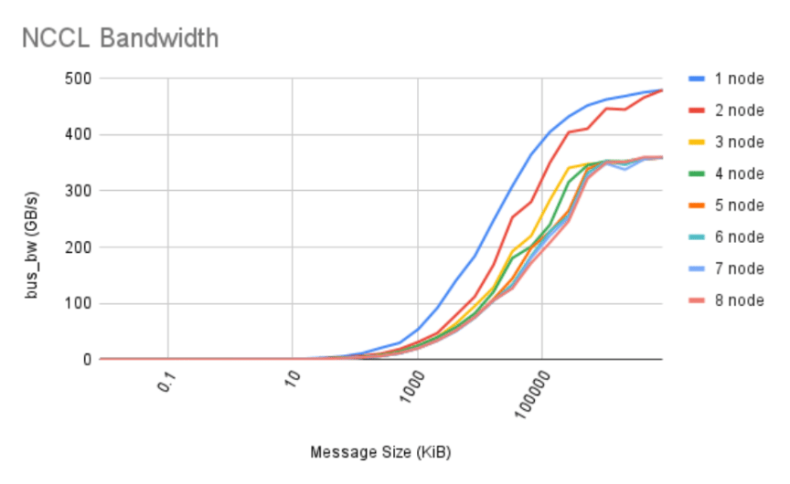
Figure: NCCL bus bandwidth test results for machines used in this report, for 1-8 nodes
Hardware and Software
DigitalOcean Bare-Metal machines
DO bare metal machines consisting of 8 H100x8 nodes and the nodes were linked by an RDMA over Converged Ethernet (RoCE) network with a common VPC, with a shared storage filesystem providing multiple terabytes of storage. Each node consisted of 8 H100 GPUs connected by NVLink, for a total of 64 GPUs. As bare-metal machines, the Ubuntu operating system was provided, and MosaicML was then run from a Docker container.
As a consequence of MosaicML’s usage of shared drives without requiring SLURM, Docker containers had to be duplicated on each node, but once done funetuning runs can be executed using a single command on each node.
The shared nature of the machines resulted in 8 of the 16 nodes being used for this project.
MosaicML LLM Foundry
This is an open source tool that allows pretraining and finetuning of models in a multinode setting. Particular positive attributes of this tool are:
- Emphasis on end-to-end usage, including data preparation, model training/finetuning, inference, and evaluation, like in real customer use cases.
- Command-line based interface that allows pretraining and finetuning to be instantiated in this setting without the requirement to write a lot of code specialized to a particular application.
- Shared disk multinode setup that avoided the need for setting up and usage of SLURM, unlike most multinode tools that introduce this complex additional overhead taken from the HPC world.
- Proof of efficient usage of GPU compute via the model FLOPS utilization (MFU) metric
- Existing benchmarks from MosaicML enabling calibration of expectations (e.g., of MFU), albeit on different machines so not 1:1 comparable with our numbers
- Support of real-world large language models in the MPT series
- Weights & Biases logging integration
Thanks for learning with the DigitalOcean Community. Check out our offerings for compute, storage, networking, and managed databases.
About the author(s)
Working with data and machine learning for 25 years. Astrophysics 2000-2012, Silicon Valley 2013-present. Interested in using my broad overview and experience of data science to help out the community.
Still looking for an answer?
This textbox defaults to using Markdown to format your answer.
You can type !ref in this text area to quickly search our full set of tutorials, documentation & marketplace offerings and insert the link!
 This work is licensed under a Creative Commons Attribution-NonCommercial- ShareAlike 4.0 International License.
Become a contributor for community
Get paid to write technical tutorials and select a tech-focused charity to receive a matching donation.

DigitalOcean Documentation
Full documentation for every DigitalOcean product.

Resources for startups and AI-native businesses
The Wave has everything you need to know about building a business, from raising funding to marketing your product.
The developer cloud
Scale up as you grow — whether you're running one virtual machine or ten thousand.

Start building today
From GPU-powered inference and Kubernetes to managed databases and storage, get everything you need to build, scale, and deploy intelligent applications.
