By Thomas Vincent and Lisa Tagliaferri

Introduction
Time series provide the opportunity to forecast future values. Based on previous values, time series can be used to forecast trends in economics, weather, and capacity planning, to name a few. The specific properties of time-series data mean that specialized statistical methods are usually required.
In this tutorial, we will aim to produce reliable forecasts of time series. We will begin by introducing and discussing the concepts of autocorrelation, stationarity, and seasonality, and proceed to apply one of the most commonly used method for time-series forecasting, known as ARIMA.
One of the methods available in Python to model and predict future points of a time series is known as SARIMAX, which stands for Seasonal AutoRegressive Integrated Moving Averages with eXogenous regressors. Here, we will primarily focus on the ARIMA component, which is used to fit time-series data to better understand and forecast future points in the time series.
Prerequisites
This guide will cover how to do time-series analysis on either a local desktop or a remote server. Working with large datasets can be memory intensive, so in either case, the computer will need at least 2GB of memory to perform some of the calculations in this guide.
To make the most of this tutorial, some familiarity with time series and statistics can be helpful.
For this tutorial, we’ll be using Jupyter Notebook to work with the data. If you do not have it already, you should follow our tutorial to install and set up Jupyter Notebook for Python 3.
Step 1 — Installing Packages
To set up our environment for time-series forecasting, let’s first move into our local programming environment or server-based programming environment:
- cd environments
- . my_env/bin/activate
From here, let’s create a new directory for our project. We will call it ARIMA and then move into the directory. If you call the project a different name, be sure to substitute your name for ARIMA throughout the guide
- mkdir ARIMA
- cd ARIMA
This tutorial will require the warnings, itertools, pandas, numpy, matplotlib and statsmodels libraries. The warnings and itertools libraries come included with the standard Python library set so you shouldn’t need to install them.
Like with other Python packages, we can install these requirements with pip.
We can now install pandas, statsmodels, and the data plotting package matplotlib. Their dependencies will also be installed:
- pip install pandas numpy statsmodels matplotlib
At this point, we’re now set up to start working with the installed packages.
Step 2 — Importing Packages and Loading Data
To begin working with our data, we will start up Jupyter Notebook:
- jupyter notebook
To create a new notebook file, select New > Python 3 from the top right pull-down menu:
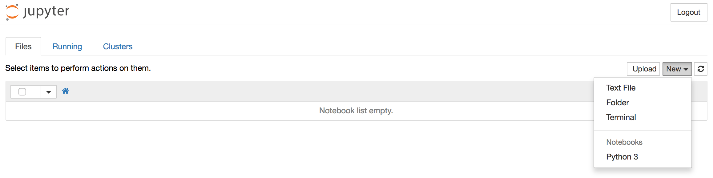
This will open a notebook.
As is best practice, start by importing the libraries you will need at the top of your notebook:
import warnings
import itertools
import pandas as pd
import numpy as np
import statsmodels.api as sm
import matplotlib.pyplot as plt
plt.style.use('fivethirtyeight')
We have also defined a matplotlib style of fivethirtyeight for our plots.
We’ll be working with a dataset called “Atmospheric CO2 from Continuous Air Samples at Mauna Loa Observatory, Hawaii, U.S.A.,” which collected CO2 samples from March 1958 to December 2001. We can bring in this data as follows:
data = sm.datasets.co2.load_pandas()
y = data.data
Let’s preprocess our data a little bit before moving forward. Weekly data can be tricky to work with since it’s a briefer amount of time, so let’s use monthly averages instead. We’ll make the conversion with the resample function. For simplicity, we can also use the fillna() function to ensure that we have no missing values in our time series.
# The 'MS' string groups the data in buckets by start of the month
y = y['co2'].resample('MS').mean()

# The term bfill means that we use the value before filling in missing values
y = y.fillna(y.bfill())

print(y)
Outputco2
1958-03-01  316.100000
1958-04-01  317.200000
1958-05-01  317.433333
...
2001-11-01  369.375000
2001-12-01  371.020000
Let’s explore this time series e as a data visualization:
y.plot(figsize=(15, 6))
plt.show()
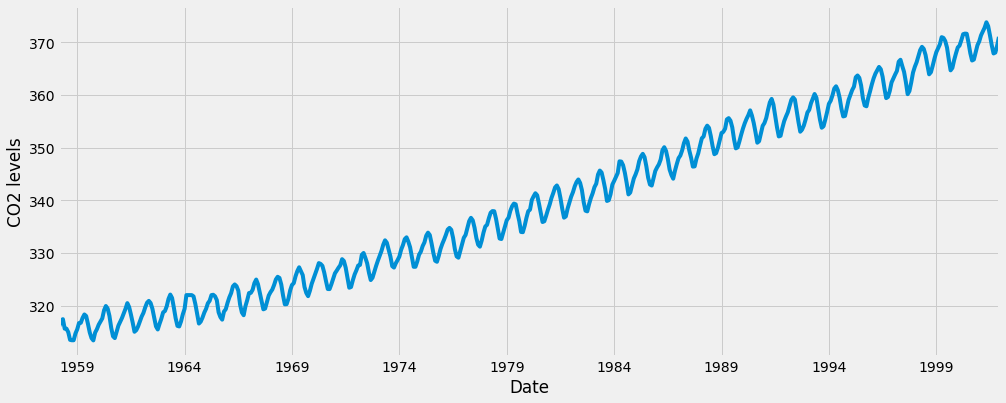
Some distinguishable patterns appear when we plot the data. The time series has an obvious seasonality pattern, as well as an overall increasing trend.
To learn more about time series pre-processing, please refer to “A Guide to Time Series Visualization with Python 3,” where the steps above are described in much more detail.
Now that we’ve converted and explored our data, let’s move on to time series forecasting with ARIMA.
Step 3 — The ARIMA Time Series Model
One of the most common methods used in time series forecasting is known as the ARIMA model, which stands for AutoregRessive Integrated Moving Average. ARIMA is a model that can be fitted to time series data in order to better understand or predict future points in the series.
There are three distinct integers (p, d, q) that are used to parametrize ARIMA models. Because of that, ARIMA models are denoted with the notation ARIMA(p, d, q). Together these three parameters account for seasonality, trend, and noise in datasets:
pis the auto-regressive part of the model. It allows us to incorporate the effect of past values into our model. Intuitively, this would be similar to stating that it is likely to be warm tomorrow if it has been warm the past 3 days.dis the integrated part of the model. This includes terms in the model that incorporate the amount of differencing (i.e. the number of past time points to subtract from the current value) to apply to the time series. Intuitively, this would be similar to stating that it is likely to be same temperature tomorrow if the difference in temperature in the last three days has been very small.qis the moving average part of the model. This allows us to set the error of our model as a linear combination of the error values observed at previous time points in the past.
When dealing with seasonal effects, we make use of the seasonal ARIMA, which is denoted as ARIMA(p,d,q)(P,D,Q)s. Here, (p, d, q) are the non-seasonal parameters described above, while (P, D, Q) follow the same definition but are applied to the seasonal component of the time series. The term s is the periodicity of the time series (4 for quarterly periods, 12 for yearly periods, etc.).
The seasonal ARIMA method can appear daunting because of the multiple tuning parameters involved. In the next section, we will describe how to automate the process of identifying the optimal set of parameters for the seasonal ARIMA time series model.
Step 4 — Parameter Selection for the ARIMA Time Series Model
When looking to fit time series data with a seasonal ARIMA model, our first goal is to find the values of ARIMA(p,d,q)(P,D,Q)s that optimize a metric of interest. There are many guidelines and best practices to achieve this goal, yet the correct parametrization of ARIMA models can be a painstaking manual process that requires domain expertise and time. Other statistical programming languages such as R provide automated ways to solve this issue, but those have yet to be ported over to Python. In this section, we will resolve this issue by writing Python code to programmatically select the optimal parameter values for our ARIMA(p,d,q)(P,D,Q)s time series model.
We will use a “grid search” to iteratively explore different combinations of parameters. For each combination of parameters, we fit a new seasonal ARIMA model with the SARIMAX() function from the statsmodels module and assess its overall quality. Once we have explored the entire landscape of parameters, our optimal set of parameters will be the one that yields the best performance for our criteria of interest. Let’s begin by generating the various combination of parameters that we wish to assess:
# Define the p, d and q parameters to take any value between 0 and 2
p = d = q = range(0, 2)

# Generate all different combinations of p, q and q triplets
pdq = list(itertools.product(p, d, q))

# Generate all different combinations of seasonal p, q and q triplets
seasonal_pdq = [(x[0], x[1], x[2], 12) for x in list(itertools.product(p, d, q))]

print('Examples of parameter combinations for Seasonal ARIMA...')
print('SARIMAX: {} x {}'.format(pdq[1], seasonal_pdq[1]))
print('SARIMAX: {} x {}'.format(pdq[1], seasonal_pdq[2]))
print('SARIMAX: {} x {}'.format(pdq[2], seasonal_pdq[3]))
print('SARIMAX: {} x {}'.format(pdq[2], seasonal_pdq[4]))
OutputExamples of parameter combinations for Seasonal ARIMA...
SARIMAX: (0, 0, 1) x (0, 0, 1, 12)
SARIMAX: (0, 0, 1) x (0, 1, 0, 12)
SARIMAX: (0, 1, 0) x (0, 1, 1, 12)
SARIMAX: (0, 1, 0) x (1, 0, 0, 12)
We can now use the triplets of parameters defined above to automate the process of training and evaluating ARIMA models on different combinations. In Statistics and Machine Learning, this process is known as grid search (or hyperparameter optimization) for model selection.
When evaluating and comparing statistical models fitted with different parameters, each can be ranked against one another based on how well it fits the data or its ability to accurately predict future data points. We will use the AIC (Akaike Information Criterion) value, which is conveniently returned with ARIMA models fitted using statsmodels. The AIC measures how well a model fits the data while taking into account the overall complexity of the model. A model that fits the data very well while using lots of features will be assigned a larger AIC score than a model that uses fewer features to achieve the same goodness-of-fit. Therefore, we are interested in finding the model that yields the lowest AIC value.
The code chunk below iterates through combinations of parameters and uses the SARIMAX function from statsmodels to fit the corresponding Seasonal ARIMA model. Here, the order argument specifies the (p, d, q) parameters, while the seasonal_order argument specifies the (P, D, Q, S) seasonal component of the Seasonal ARIMA model. After fitting each SARIMAX()model, the code prints out its respective AIC score.
warnings.filterwarnings("ignore") # specify to ignore warning messages

for param in pdq:
    for param_seasonal in seasonal_pdq:
        try:
            mod = sm.tsa.statespace.SARIMAX(y,
                                            order=param,
                                            seasonal_order=param_seasonal,
                                            enforce_stationarity=False,
                                            enforce_invertibility=False)

            results = mod.fit()

            print('ARIMA{}x{}12 - AIC:{}'.format(param, param_seasonal, results.aic))
        except:
            continue
Because some parameter combinations may lead to numerical misspecifications, we explicitly disabled warning messages in order to avoid an overload of warning messages. These misspecifications can also lead to errors and throw an exception, so we make sure to catch these exceptions and ignore the parameter combinations that cause these issues.
The code above should yield the following results, this may take some time:
OutputSARIMAX(0, 0, 0)x(0, 0, 1, 12) - AIC:6787.3436240402125
SARIMAX(0, 0, 0)x(0, 1, 1, 12) - AIC:1596.711172764114
SARIMAX(0, 0, 0)x(1, 0, 0, 12) - AIC:1058.9388921320026
SARIMAX(0, 0, 0)x(1, 0, 1, 12) - AIC:1056.2878315690562
SARIMAX(0, 0, 0)x(1, 1, 0, 12) - AIC:1361.6578978064144
SARIMAX(0, 0, 0)x(1, 1, 1, 12) - AIC:1044.7647912940095
...
...
...
SARIMAX(1, 1, 1)x(1, 0, 0, 12) - AIC:576.8647112294245
SARIMAX(1, 1, 1)x(1, 0, 1, 12) - AIC:327.9049123596742
SARIMAX(1, 1, 1)x(1, 1, 0, 12) - AIC:444.12436865161305
SARIMAX(1, 1, 1)x(1, 1, 1, 12) - AIC:277.7801413828764
The output of our code suggests that SARIMAX(1, 1, 1)x(1, 1, 1, 12) yields the lowest AIC value of 277.78. We should therefore consider this to be optimal option out of all the models we have considered.
Step 5 — Fitting an ARIMA Time Series Model
Using grid search, we have identified the set of parameters that produces the best fitting model to our time series data. We can proceed to analyze this particular model in more depth.
We’ll start by plugging the optimal parameter values into a new SARIMAX model:
mod = sm.tsa.statespace.SARIMAX(y,
                                order=(1, 1, 1),
                                seasonal_order=(1, 1, 1, 12),
                                enforce_stationarity=False,
                                enforce_invertibility=False)

results = mod.fit()

print(results.summary().tables[1])
Output==============================================================================
                 coef    std err          z      P>|z|      [0.025      0.975]
------------------------------------------------------------------------------
ar.L1          0.3182      0.092      3.443      0.001       0.137       0.499
ma.L1         -0.6255      0.077     -8.165      0.000      -0.776      -0.475
ar.S.L12       0.0010      0.001      1.732      0.083      -0.000       0.002
ma.S.L12      -0.8769      0.026    -33.811      0.000      -0.928      -0.826
sigma2         0.0972      0.004     22.634      0.000       0.089       0.106
==============================================================================
The summary attribute that results from the output of SARIMAX returns a significant amount of information, but we’ll focus our attention on the table of coefficients. The coef column shows the weight (i.e. importance) of each feature and how each one impacts the time series. The P>|z| column informs us of the significance of each feature weight. Here, each weight has a p-value lower or close to 0.05, so it is reasonable to retain all of them in our model.
When fitting seasonal ARIMA models (and any other models for that matter), it is important to run model diagnostics to ensure that none of the assumptions made by the model have been violated. The plot_diagnostics object allows us to quickly generate model diagnostics and investigate for any unusual behavior.
results.plot_diagnostics(figsize=(15, 12))
plt.show()
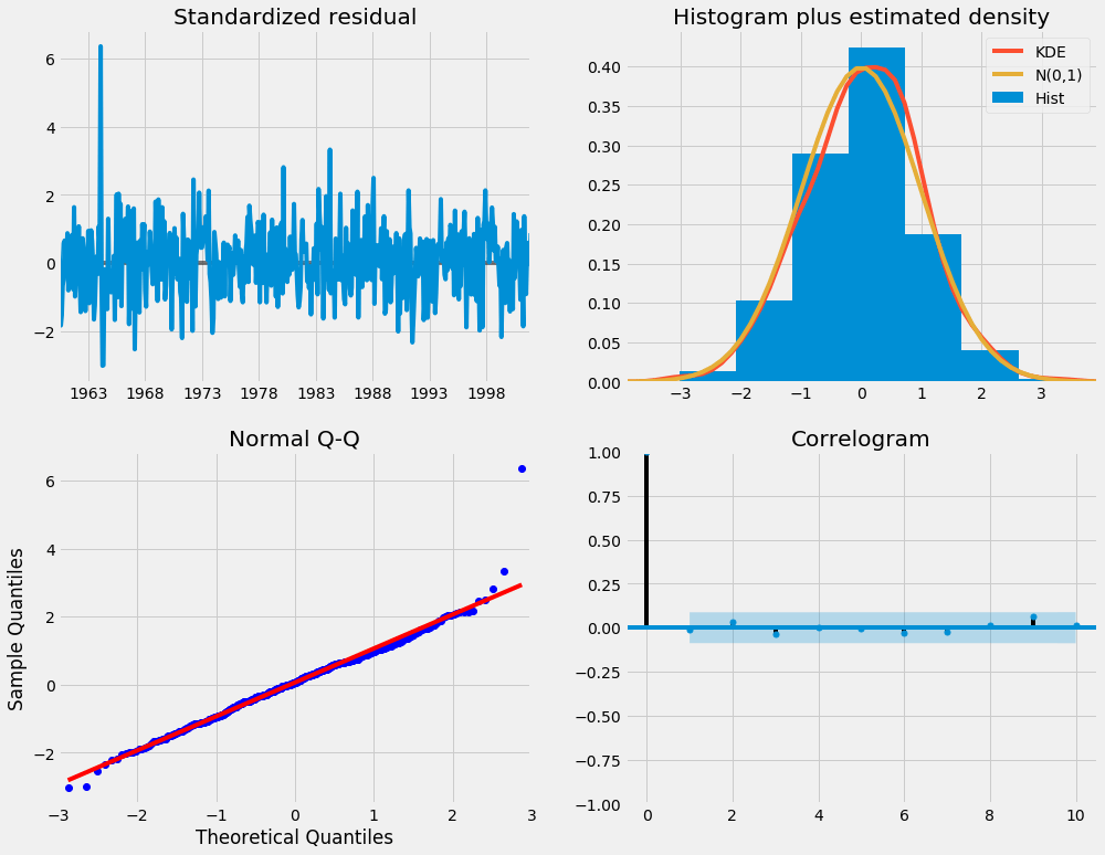
Our primary concern is to ensure that the residuals of our model are uncorrelated and normally distributed with zero-mean. If the seasonal ARIMA model does not satisfy these properties, it is a good indication that it can be further improved.
In this case, our model diagnostics suggests that the model residuals are normally distributed based on the following:
-
In the top right plot, we see that the red
KDEline follows closely with theN(0,1)line (whereN(0,1)) is the standard notation for a normal distribution with mean0and standard deviation of1). This is a good indication that the residuals are normally distributed. -
The qq-plot on the bottom left shows that the ordered distribution of residuals (blue dots) follows the linear trend of the samples taken from a standard normal distribution with
N(0, 1). Again, this is a strong indication that the residuals are normally distributed. -
The residuals over time (top left plot) don’t display any obvious seasonality and appear to be white noise. This is confirmed by the autocorrelation (i.e. correlogram) plot on the bottom right, which shows that the time series residuals have low correlation with lagged versions of itself.
Those observations lead us to conclude that our model produces a satisfactory fit that could help us understand our time series data and forecast future values.
Although we have a satisfactory fit, some parameters of our seasonal ARIMA model could be changed to improve our model fit. For example, our grid search only considered a restricted set of parameter combinations, so we may find better models if we widened the grid search.
Step 6 — Validating Forecasts
We have obtained a model for our time series that can now be used to produce forecasts. We start by comparing predicted values to real values of the time series, which will help us understand the accuracy of our forecasts. The get_prediction() and conf_int() attributes allow us to obtain the values and associated confidence intervals for forecasts of the time series.
pred = results.get_prediction(start=pd.to_datetime('1998-01-01'), dynamic=False)
pred_ci = pred.conf_int()
The code above requires the forecasts to start at January 1998.
The dynamic=False argument ensures that we produce one-step ahead forecasts, meaning that forecasts at each point are generated using the full history up to that point.
We can plot the real and forecasted values of the CO2 time series to assess how well we did. Notice how we zoomed in on the end of the time series by slicing the date index.
ax = y['1990':].plot(label='observed')
pred.predicted_mean.plot(ax=ax, label='One-step ahead Forecast', alpha=.7)

ax.fill_between(pred_ci.index,
                pred_ci.iloc[:, 0],
                pred_ci.iloc[:, 1], color='k', alpha=.2)

ax.set_xlabel('Date')
ax.set_ylabel('CO2 Levels')
plt.legend()

plt.show()
Overall, our forecasts align with the true values very well, showing an overall increase trend.
It is also useful to quantify the accuracy of our forecasts. We will use the MSE (Mean Squared Error), which summarizes the average error of our forecasts. For each predicted value, we compute its distance to the true value and square the result. The results need to be squared so that positive/negative differences do not cancel each other out when we compute the overall mean.
y_forecasted = pred.predicted_mean
y_truth = y['1998-01-01':]

# Compute the mean square error
mse = ((y_forecasted - y_truth) ** 2).mean()
print('The Mean Squared Error of our forecasts is {}'.format(round(mse, 2)))
OutputThe Mean Squared Error of our forecasts is 0.07
The MSE of our one-step ahead forecasts yields a value of 0.07, which is very low as it is close to 0. An MSE of 0 would that the estimator is predicting observations of the parameter with perfect accuracy, which would be an ideal scenario but it not typically possible.
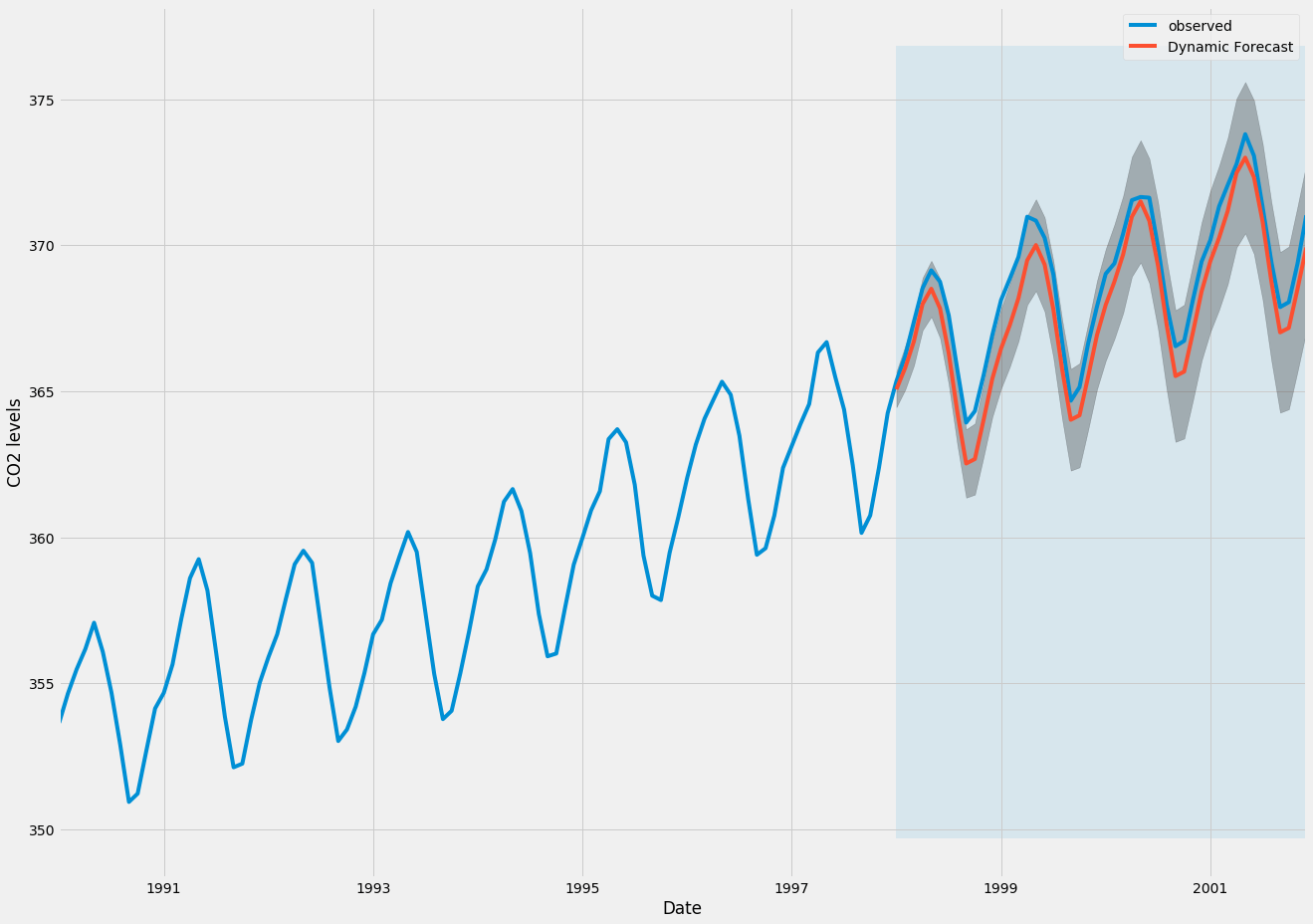
However, a better representation of our true predictive power can be obtained using dynamic forecasts. In this case, we only use information from the time series up to a certain point, and after that, forecasts are generated using values from previous forecasted time points.
In the code chunk below, we specify to start computing the dynamic forecasts and confidence intervals from January 1998 onwards.
pred_dynamic = results.get_prediction(start=pd.to_datetime('1998-01-01'), dynamic=True, full_results=True)
pred_dynamic_ci = pred_dynamic.conf_int()
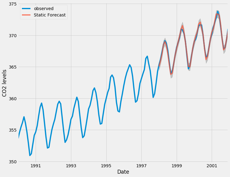
Plotting the observed and forecasted values of the time series, we see that the overall forecasts are accurate even when using dynamic forecasts. All forecasted values (red line) match pretty closely to the ground truth (blue line), and are well within the confidence intervals of our forecast.
ax = y['1990':].plot(label='observed', figsize=(20, 15))
pred_dynamic.predicted_mean.plot(label='Dynamic Forecast', ax=ax)

ax.fill_between(pred_dynamic_ci.index,
                pred_dynamic_ci.iloc[:, 0],
                pred_dynamic_ci.iloc[:, 1], color='k', alpha=.25)

ax.fill_betweenx(ax.get_ylim(), pd.to_datetime('1998-01-01'), y.index[-1],
                 alpha=.1, zorder=-1)

ax.set_xlabel('Date')
ax.set_ylabel('CO2 Levels')

plt.legend()
plt.show()
Once again, we quantify the predictive performance of our forecasts by computing the MSE:
# Extract the predicted and true values of our time series
y_forecasted = pred_dynamic.predicted_mean
y_truth = y['1998-01-01':]

# Compute the mean square error
mse = ((y_forecasted - y_truth) ** 2).mean()
print('The Mean Squared Error of our forecasts is {}'.format(round(mse, 2)))
OutputThe Mean Squared Error of our forecasts is 1.01
The predicted values obtained from the dynamic forecasts yield an MSE of 1.01. This is slightly higher than the one-step ahead, which is to be expected given that we are relying on less historical data from the time series.
Both the one-step ahead and dynamic forecasts confirm that this time series model is valid. However, much of the interest around time series forecasting is the ability to forecast future values way ahead in time.
Step 7 — Producing and Visualizing Forecasts
In the final step of this tutorial, we describe how to leverage our seasonal ARIMA time series model to forecast future values. The get_forecast() attribute of our time series object can compute forecasted values for a specified number of steps ahead.
# Get forecast 500 steps ahead in future
pred_uc = results.get_forecast(steps=500)

# Get confidence intervals of forecasts
pred_ci = pred_uc.conf_int()
We can use the output of this code to plot the time series and forecasts of its future values.
ax = y.plot(label='observed', figsize=(20, 15))
pred_uc.predicted_mean.plot(ax=ax, label='Forecast')
ax.fill_between(pred_ci.index,
                pred_ci.iloc[:, 0],
                pred_ci.iloc[:, 1], color='k', alpha=.25)
ax.set_xlabel('Date')
ax.set_ylabel('CO2 Levels')

plt.legend()
plt.show()

Both the forecasts and associated confidence interval that we have generated can now be used to further understand the time series and foresee what to expect. Our forecasts show that the time series is expected to continue increasing at a steady pace.
As we forecast further out into the future, it is natural for us to become less confident in our values. This is reflected by the confidence intervals generated by our model, which grow larger as we move further out into the future.
Conclusion
In this tutorial, we described how to implement a seasonal ARIMA model in Python. We made extensive use of the pandas and statsmodels libraries and showed how to run model diagnostics, as well as how to produce forecasts of the CO2 time series.
Here are a few other things you could try:
- Change the start date of your dynamic forecasts to see how this affects the overall quality of your forecasts.
- Try more combinations of parameters to see if you can improve the goodness-of-fit of your model.
- Select a different metric to select the best model. For example, we used the
AICmeasure to find the best model, but you could seek to optimize the out-of-sample mean square error instead.
For more practice, you could also try to load another time series dataset to produce your own forecasts.
Thanks for learning with the DigitalOcean Community. Check out our offerings for compute, storage, networking, and managed databases.
Tutorial Series: Time Series Visualization and Forecasting
Time series are a pivotal component of data analysis. This series goes through how to handle time series visualization and forecasting in Python 3.
About the author(s)
Statistician & data scientist. Strong background in whiskey.
Community and Developer Education expert. Former Senior Manager, Community at DigitalOcean. Focused on topics including Ubuntu 22.04, Ubuntu 20.04, Python, Django, and more.
Still looking for an answer?
This textbox defaults to using Markdown to format your answer.
You can type !ref in this text area to quickly search our full set of tutorials, documentation & marketplace offerings and insert the link!
Hi! Thanks for sharing this. I was trying to forecast hourly values. The seasonality to capture should be similar as the 168th previous value. This means, Friday 9PM of this week should be similar than Friday 9PM of the past week. That is why I decided to use 168 seasionality (24*7) but it takes very long and consumes lots of memory. I’ve tried several times using 7 and 24 seasionality but it wasn’t doing it well when forecasting (previous fitting with dynamic set to False was working perfectly). Do you have any advice for this situation? Thanks in advance.
Thanks for the Guide.
I tried this with my own data. And at the model result summary part, I got ma.L1 having p-value over 0.88. So, I definitely want to get rid of this feature from the model. But how do I do that? How to remove a feature from the model??
very nice tutorial. thanks! I am a new one to ARIMA model, I want to ask you some questions.
-
I found you use all the historical data to fit an ARIMA Time Series Model, and use part of all the historical data to validate mode, with code: pred = results.get_prediction(start=pd.to_datetime(‘1998-01-01’), dynamic=False) pred_ci = pred.conf_int() But why the data to validate model is one part of data for fitting model before. You know in machine learning, the train data and test data is split, I don’t why here is different.
-
how about data stationary, could you tell me why you set the enforce_stationary is false.
-
how about days data not month data(average) for fit mode to predict, how about week data for prediction, could you tell me how to do it
thanks!
I got an error on line: pred = results.get_prediction(start=pd.to_datetime(‘1998-02-01’), dynamic=False)
File “pandas_libs\tslib.pyx”, line 1080, in pandas._libs.tslib._Timestamp.richcmp (pandas_libs\tslib.c:20281) TypeError: Cannot compare type ‘Timestamp’ with type ‘int’
How can I solve it?
Hi. Thank you so much for your wonderful sharing. Is there are any way to catch the minimum value of AIC automatically? It would be wonderful, if the best set for ARIMAX was stored on a external variable and pass them to next step. Is it possible? how? Thanks you
The line “results = mod.fit()” prints a lot of stuff to the console for me, making it difficult to find the best combination
Hi,
Thanks for such post. Could you please help me understanding the use of exogenous variables ? I don’t see any use of such independent variables here.
Hi, awesome work here, but I’m having issues with my data set…when i use your code it gives me errors on the data and time, how did u deal with this stuff?
PS: I have converted to string, float, datatime etc but keep getting errors at the step 5
SARIMAX has a score method. Can you please help to explain the kind of parameters that should be fed into it, and how do we interpret the scores ?
Thanks for neat tutorial on ARIMA forcasting model One help
- While excuting this line: pred_uc = results.get_forecast(steps=500)
<statsmodels.tsa.statespace.mlemodel.PredictionResultsWrapper object at 0x0000000015369DD8> the data which is predicted is stored as objects and is there any way that i can exctract that in the form of array or dataframe Thanks in advance…
 This work is licensed under a Creative Commons Attribution-NonCommercial- ShareAlike 4.0 International License.
Become a contributor for community
Get paid to write technical tutorials and select a tech-focused charity to receive a matching donation.

DigitalOcean Documentation
Full documentation for every DigitalOcean product.

Resources for startups and AI-native businesses
The Wave has everything you need to know about building a business, from raising funding to marketing your product.
The developer cloud
Scale up as you grow — whether you're running one virtual machine or ten thousand.

Start building today
From GPU-powered inference and Kubernetes to managed databases and storage, get everything you need to build, scale, and deploy intelligent applications.
