Anomaly Detection in Python with Isolation Forest

Anomaly detection plays a key role in many real-world applications—from catching fraudulent transactions in banking to predicting equipment failures in industrial systems. It helps identify unusual patterns or outliers in data that may indicate critical issues or hidden insights. One of the most effective yet easy-to-use algorithms for this task is Isolation Forest.

It works by isolating anomalies instead of profiling normal data, making it fast and efficient even on large datasets. In this article, we’ll explore what anomaly detection is, where it’s used, how the Isolation Forest algorithm works, and how you can implement it in Python with a practical example. Whether you’re new to machine learning or just looking to sharpen your skills, this guide will walk you through the essentials in a simple, hands-on way.

Prerequisites

In order to follow along with this article, you need experience with Python code and a beginner’s understanding of Deep Learning. We will operate under the assumption that all readers have access to sufficiently powerful machines, so they can run the code provided. If you do not have access to a GPU, we suggest using DigitalOcean GPU Droplets.

If you’re new to Python, check out this introductory guide to help you set up your system and get ready to run basic coding examples.

Introduction to Anomaly Detection

An outlier is nothing but a data point that differs significantly from other data points in the given dataset.

Anomaly detection is the process of finding the outliers in the data, i.e., points that are significantly different from the majority of the other data points.

Large, real-world datasets may have very complicated patterns that are difficult to detect by just looking at the data. That’s why the study of anomaly detection is an extremely important application of Machine Learning.

In this article, we will implement anomaly detection using the isolation forest algorithm. We have a simple dataset of salaries, and a few of the salaries are anomalous. Our goal is to find those salaries. You could imagine a situation where certain employees in a company are making an unusually large sum of money, which might be an indicator of unethical activity.

Before we proceed with the implementation, let’s discuss some of the use cases of anomaly detection.

Anomaly Detection Use Cases

Anomaly detection has wide applications across industries. Below are some of the popular use cases:

Banking. Finding abnormally high deposits. Every account holder generally has certain patterns of depositing money into their account. If there is an outlier to this pattern, the bank needs to be able to detect and analyze it, e.g., for money laundering.

Finance. Finding the pattern of fraudulent purchases. Every person generally has certain patterns of purchases. If there is an outlier to this pattern, the bank needs to detect it in order to analyze it for potential fraud.

Healthcare. Detecting fraudulent insurance claims and payments.

Manufacturing. Abnormal machine behavior can be monitored for cost control. Many companies continuously monitor the input and output parameters of the machines they own. It is a well-known fact that before failure a machine shows abnormal behaviors in terms of these input or output parameters. A machine needs to be constantly monitored for anomalous behavior from the perspective of preventive maintenance.

Networking. Detecting intrusion into networks. Any network exposed to the outside world faces this threat. Intrusions can be detected early on using monitoring for anomalous activity in the network.

Now, let’s understand what the isolation forest algorithm in machine learning is.

What Is Isolation Forest?

Isolation forest is an unsupervised machine learning algorithm for anomaly detection. It identifies anomalies by isolating outliers in the data.

Isolation Forest is based on the Decision Tree algorithm. It isolates the outliers by randomly selecting a feature from the given set of features and then randomly selecting a split value between the max and min values of that feature. This random partitioning of features will produce shorter paths in trees for the anomalous data points, thus distinguishing them from the rest of the data.

In general, the first step to anomaly detection is to construct a profile of what’s “normal” and then report anything that cannot be considered normal as anomalous. However, the isolation forest algorithm does not work on this principle; it does not first define “normal” behavior and does not calculate point-based distances.

As you might expect from the name, Isolation Forest instead works by isolating anomalies, explicitly isolating anomalous points in the dataset.

The Isolation Forest algorithm is based on the principle that anomalies are observations that are few and different, which should make them easier to identify. Isolation Forest uses an ensemble of Isolation Trees for the given data points to isolate anomalies.

Isolation Forest recursively generates partitions on the dataset by randomly selecting a feature and then randomly selecting a split value for the feature. Presumably, the anomalies need fewer random partitions to be isolated compared to “normal” points in the dataset, so the anomalies will be the points with a smaller path length in the tree, path length being the number of edges traversed from the root node.

Using Isolation Forest, we can not only detect anomalies faster, but we also require less memory compared to other algorithms.

Isolation Forest isolates anomalies in the data points instead of profiling normal data points. As anomaly data points mostly have a lot shorter tree paths than the normal data points, trees in the Isolation Forest do not need to have a large depth, so a smaller max_depth can be used, resulting in low memory requirement.

This algorithm works very well with a small data set as well.

Let’s do some exploratory data analysis now to get an idea about the given data.

Exploratory Data Analysis

Let’s import the required libraries first. We are importing numpy, pandas, seaborn and matplotlib. Apart form that we also need to import IsolationForest from sklearn.ensemble.

import numpy as np
import pandas as pd
import seaborn as sns
import matplotlib.pyplot as plt
from sklearn.ensemble import IsolationForest

Once the libraries are imported, we need to read the data from the CSV into the pandas data frame and check the first 10 rows of data.

The data is a collection of salaries, in USD per year, of different professionals. This data has few anomalies (like salary too high or too low) which we will be detecting.

df = pd.read_csv('salary.csv')
df.head(10)

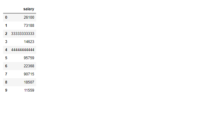
Dataset head

To get more of an idea of the data we have plotted a violin plot of salary data as shown below. A violin plot is a method of plotting numeric data.

Typically a violin plot includes all the data that is in a box plot, a marker for the median of the data, a box or marker indicating the interquartile range, and possibly all sample points, if the number of samples is not too high.

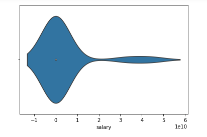
Violin Plot for Salary

To get a better idea of outliers, we may also like to look at a box plot. This is also known as a box-and-whisker plot. The box in a box plot shows the quartiles of the dataset, while the whiskers show the rest of the distribution.

Whiskers do not show the points that are determined to be outliers. Outliers are detected by a method that is a function of the interquartile range. In statistics, the interquartile range, also known as midspread or middle 50%, is a measure of statistical dispersion, equal to the difference between the 75th and 25th percentiles.

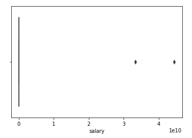
Box Plot for Salary, indicating the two outliers on the right

Once we have completed our exploratory data analysis, it’s time to define and fit the model.

Define and Fit Model

We’ll create a model variable and instantiate the IsolationForest class. We are passing the values of four parameters to the Isolation Forest method, listed below.

Number of estimators: n_estimators refers to the number of base estimators or trees in the ensemble, i.e., the number of trees that will get built in the forest. This is an integer parameter and is optional. The default value is 100.

Max samples: max_samples is the number of samples to be drawn to train each base estimator. If max_samples is more than the number of samples provided, all samples will be used for all trees. The default value of max_samples is ‘auto’. If ‘auto’, then max_samples=min(256, n_samples)

Contamination: This is a parameter that the algorithm is quite sensitive to; it refers to the expected proportion of outliers in the dataset. This is used when fitting to define the threshold on the scores of the samples. The default value is ‘auto’. If ‘auto’, the threshold value will be determined as in the original paper of Isolation Forest.

Max features: All the base estimators are not trained with all the features available in the dataset. It is the number of features to draw from the total features to train each base estimator or tree.The default value of max features is one.

model=IsolationForest(n_estimators=50, max_samples='auto', contamination=float(0.1),max_features=1.0)
model.fit(df[['salary']])

Isolation Forest Model Training Output

After we defined the model above we need to train the model using the data given. For this we are using the fit() method as shown above. This method is passed one parameter, which is our data of interest (in this case, the salary column of the dataset).

Once the model is trained properly it will output the IsolationForest instance as shown in the output of the cell above.

Now is the time to add the scores and anomaly column of the dataset.

Add Scores and Anomaly Column

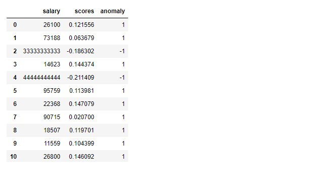
After the model is defined and fit, let’s find the scores and anomaly column. We can find out the values of the scores column by calling decision_function() of the trained model and passing the salary as a parameter.

Similarly we can find the values of anomaly column by calling the predict() function of the trained model and passing the salary as parameter.

These columns are going to be added to the data frame df. After adding these two columns let’s check the data frame. As expected, the data frame has three columns now: salary, scores and anomaly. A negative score value and a -1 for the value of anomaly columns indicate the presence of anomaly. A value of 1 for the anomaly represents the normal data.

Each data point in the training set is assigned an anomaly score by this algorithm. We can define a threshold, and using the anomaly score, it may be possible to mark a data point as anomalous if its score is greater than the predefined threshold.

df['scores']=model.decision_function(df[['salary']])
df['anomaly']=model.predict(df[['salary']])
df.head(20)

Added scores and Anomaly Column for Isolation Forest

After adding the scores and anomalies for all the rows in the data, we will print the predicted anomalies.

Print Anomalies

To print the predicted anomalies in the data we need to analyse the data after addition of scores and anomaly column. As you can see above for the predicted anomalies the anomaly column values would be -1 and their scores will be negative.

Using this information, we can print the predicted anomaly (two data points in this case) as below.

anomaly=df.loc[df['anomaly']==-1]
anomaly_index=list(anomaly.index)
print(anomaly)

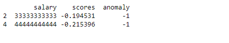
Anomaly output

Note that we could print not only the anomalous values but also their index in the dataset, which is useful information for further processing.

Evaluating the model

For evaluating the model let’s set a threshold as salary > 99999 is an outlier.Let us find out the number of outlier present in the data as per the above rule using code as below.

outliers_counter = len(df[df['salary'] > 99999])
outliers_counter

outlier_counter = 2

Let us calculate the accuracy of the model by finding how many outliers the model found divided by how many outliers are present in the data.

print("Accuracy percentage:", 100*list(df['anomaly']).count(-1)/(outliers_counter))

Accuracy percentage: 100 %

Conclusion

In this tutorial, we explored the fundamentals of anomaly detection and how the Isolation Forest algorithm can effectively identify outliers in a dataset. Along the way, we visualized our data using exploratory tools like box plots and violin plots, which helped us understand the distribution and spot anomalies more intuitively. We then implemented Isolation Forest in Python and successfully detected the real outliers in our sample dataset.

If you’re planning to integrate anomaly detection into a real-world application—whether it’s fraud detection, server monitoring, or predictive maintenance—Isolation Forest offers a scalable and efficient solution. You can easily deploy and scale your machine learning workflows using DigitalOcean Droplets or take advantage of DigitalOcean’s 1-Click ML Models to accelerate your development process.

We hope you found this article helpful and that it becomes a useful reference for your future projects. Happy coding and stay curious!