AI Technical Writer

Ever wondered how machines make decisions that feel almost human? A lot of classical machine learning models is based on an algorithm known as Decision Trees. One of the most intuitive yet powerful tools in machine learning. They serve as the foundation for many popular algorithms like Random Forests, Bagging, and Boosted Trees, which are widely used in real-world applications such as fraud detection, medical diagnosis, and customer segmentation.
The concept of decision trees was introduced by Leo Breiman, a renowned statistician at the University of California, Berkeley. He proposed a method where data is represented as a branching tree structure: each internal node tests a specific feature or condition, each branch shows the result of that test, and each leaf node makes a final prediction — either a class label (for classification) or a value (for regression).
In fact, when you hear the term CART (Classification and Regression Trees), it’s just another name for decision trees. In this article, we’ll explain how decision trees work, how they’re constructed, and how to implement them in Python using real-world data. In this article, we’ll cover the following modules:
- What are Decision Trees?
- Why Decision Trees?
- Types of Decision Trees
- Key Terminologies
- How to Create a Decision Tree
- Gini Impurity
- Chi-Square
- Information Gain
- Applications of Decision Trees
- The Hyperparameters
- Code Demonstration
- Advantages and Disadvantages of Decision Trees
- Summary and Conclusions
What are Decision Trees?
Decision Tree refers to a tree-like structure that tries to mimic human decision making by splitting the data into smaller and smaller sub-groups based on certain decision criteria or certain rules. The tree is made up of certain series of yes/no questions or conditional statements about the features from the data to reach conclusions like classifying an email spam or not spam or predicting a house price.
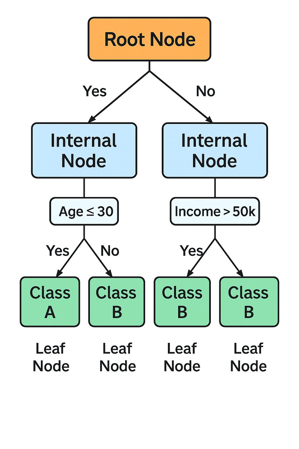
Basic Components:
- Root Node: The starting point of the tree, which also represents the entire dataset.
- Internal Nodes: Each of the internal nodes asks a question about a feature (e.g., “Is age > 30?”).
- Branches: The possible outcomes of a question (e.g., Yes or No).
- Leaf Nodes: The final output or prediction (e.g., Class A, Class B, or a number).
Why Decision Trees?
Tree-based algorithms are a widely used family of supervised machine learning techniques designed for both classification and regression tasks. These methods are non-parametric, meaning they don’t make assumptions about the underlying data distribution or a fixed number of parameters. In contrast, parametric models (like linear regression) rely on a predetermined form and a fixed set of parameters, making them less flexible but often simpler.
If you’re new to supervised learning, it refers to training models using labeled data — that is, data where the input features are paired with known output labels. This allows the algorithm to learn patterns and adjust its predictions by comparing them to the correct answers during training.
A decision tree resembles an upside-down tree. It starts with a root node that contains an initial decision rule. From there, the tree branches out into internal nodes, each representing further decision rules—for example, “Does the person exercise regularly?” Eventually, the tree reaches leaf nodes, which contain no further rules and instead represent final predictions or outcomes.
Before we dive deeper, let’s take a quick look at the different types of decision trees and how they’re applied in machine learning.
Types of Decision Trees
Decision Trees are classified into two types, based on the target variables.
- Categorical Variable Decision Trees: This is where the algorithm has a categorical target variable. For example, consider you are asked to predict the relative price of a computer as one of three categories: low, medium, or high. Features could include monitor type, speaker quality, RAM, and SSD. The decision tree will learn from these features, and after passing each data point through each node, it will end up at a leaf node of one of the three categorical targets: low, medium, or high.
- Continuous Variable Decision Trees: In this case, the features input to the decision tree (e.g., qualities of a house) will be used to predict a continuous output (e.g., the price of that house).
Key Terminology
Every tree has a root node, where the inputs are passed through. This root node is further divided into sets of decision nodes where results and observations are conditionally based. The process of dividing a single node into multiple nodes is called splitting. If a node doesn’t split into further nodes, then it’s called a leaf node, or terminal node. A subsection of a decision tree is called a branch or sub-tree (e.g., in the box in the image below).
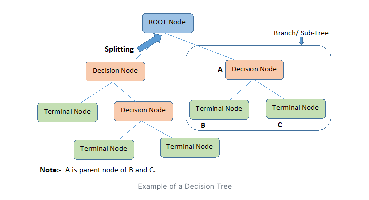
There’s also an important concept that works in the opposite direction of splitting: it’s called pruning. Instead of growing the tree by adding more decision rules, pruning involves removing unnecessary or less important rules from the tree. This helps reduce the tree’s complexity, making the model more efficient and less prone to overfitting.
Now that we have a solid understanding of what a decision tree looks like and how it functions, let’s explore the process of splitting and learn how to build a decision tree from scratch.
How To Create a Decision Tree
In this section, we shall discuss the core algorithms describing how decision trees are created. These algorithms are completely dependent on the target variable; however, they vary from the algorithms used for classification and regression trees.
Several techniques are used to decide how to split the given data. The main goal of decision trees is to make the best splits between nodes, which will optimally divide the data into the correct categories. To do this, we need to use the right decision rules, which directly affect the algorithm’s performance.
There are some assumptions that need to be considered before we get started:
- In the beginning, the whole data is considered as the root, thereafter, we use the algorithms to make a split or divide the root into subtrees.
- The feature values are considered to be categorical. If the values are continuous, then they are separated prior to building the model.
- Records are distributed recursively on the basis of attribute values.
- The ordering of attributes as root or internal node of the tree is done using a statistical approach.
Let’s get started with the commonly used techniques to split, and thereby, construct the Decision tree.
Gini Impurity
In an ideal scenario, if all the data points at a node belong to a single class, that node is said to be pure. However, this is rarely the case in real-world datasets. To quantify how impure or mixed a node is, we use a metric called Gini impurity (pronounced “jee-nee”).
Gini impurity measures the probability that a randomly selected sample would be incorrectly classified if it were randomly labeled according to the distribution of labels in that node. The idea is simple: the purer the node, the lower the impurity — and vice versa.
Key Characteristics of Gini Impurity:
-
The value ranges between 0 and 1:
- 0 means perfect purity — all samples at that node belong to one class.
- 1 means maximum impurity — samples are evenly distributed among all classes.
- A score of 0.5 typically suggests a 50-50 split between two classes — the node is moderately impure.
-
It’s considered an impurity metric because it tells us how “unclean” or mixed the class labels are at a particular split. The goal in decision trees is to find splits that minimize impurity.
-
Gini impurity is fast to compute and is the default splitting criterion in many tree-based algorithms, such as CART (Classification and Regression Trees).
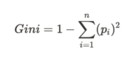
Where pi is the probability of a particular element belonging to a specific class. Now, let’s take a look at the pseudo-code for calculating and building a decision tree using the Gini Impurity measure as our guide.
Gini Index:
    for each branch in a split:
        Calculate percent branch represents  # Used for weighting
        for each class in-branch:
            Calculate the probability of that class in the given branch
            Square the class probability
        Sum the squared class probabilities
        Subtract the sum from 1  # This is the Gini Index for that branch
    Weight each branch based on the baseline probability
    Sum the weighted Gini index for each split
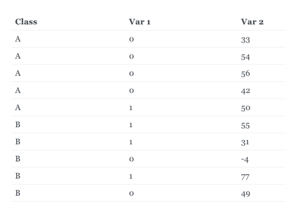
We’ll now look at a simple example explaining the above algorithm. Consider the following table of data, where for each element (row) we have two variables describing it, and an associated class label.
Gini Index Example:
Here’s a clear, step-by-step explanation and reformatted version of your Gini index calculation for a split on Var1, along with some context to make it easier to understand:
Step-by-Step Gini Index Calculation for a Split on Var1
Let’s say we have a dataset with 10 total instances, and we are evaluating a split based on the feature Var1.
Step 1: Understand the Distribution
Var1 == 1occurs 4 times → 4/10 = 40% of the dataVar1 == 0occurs 6 times → 6/10 = 60% of the data
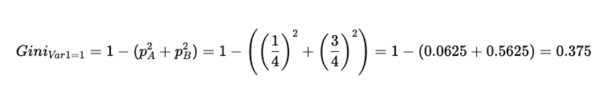
Step 2: Calculate Gini Impurity for Each Split
For Var1 == 1:
- Class A: 1 out of 4 instances → pA = 1/4
- Class B: 3 out of 4 instances → pB = 3/4
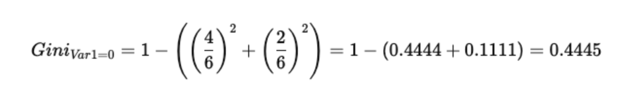
For Var1 == 0:
- Class A: 4 out of 6 instances → pA = 4/6
- Class B: 2 out of 6 instances → pB = 2/6
Step 3: Compute Weighted Gini for the Split
Each Gini score is weighted by the proportion of the dataset it represents:
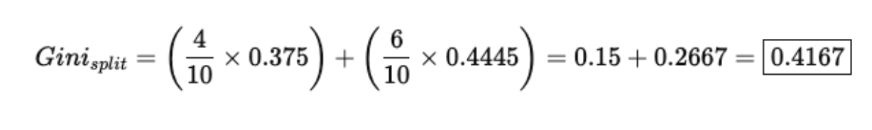
Final Result:
Weighted Gini Index for the split on Var1 = 0.4167
A lower Gini value indicates a better split (more class purity), so this value can be compared to splits on other variables to determine the best feature to split on.
Information Gain
Information Gain depicts the amount of information that is gained by an attribute. It tells us how important the attribute is. Since Decision Tree construction is all about finding the right split node that assures high accuracy, Information Gain is all about finding the best nodes that return the highest information gain. This is computed using a factor known as Entropy. Entropy defines the degree of disorganization in a system. The more disorganized the system is, the greater the entropy. When the sample is wholly homogeneous, then the entropy turns out to be zero, and if the sample is partially organized, say 50% of it is organized, then the entropy turns out to be one.
This acts as the base factor in determining the information gain. Entropy and Information Gain together are used to construct the Decision Tree, and the algorithm is known as ID3.
Let’s understand the step-by-step procedure that’s used to calculate the Information Gain, and thereby, construct the Decision tree.
- Calculate the entropy of the output attribute (before the split) using the formula.
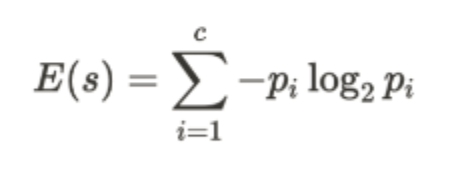
In this case, p represents the probability of success, and q represents the probability of failure at a node. For example, if we have 10 data points where 5 are labeled True and 5 are labeled False, then the number of classes, c, is 2. The probabilities for each class, p₁ and p₂, are both equal to ½.
- Calculate the entropy of all the input attributes using the formula.
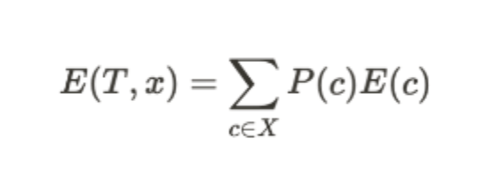
T is the output attribute, X is the input attribute,
P© is the probability w.r.t the possible data point present at X, and E© is the entropy w.r.t ‘True’ pertaining to the possible data point. Let’s consider an input attribute called priority, which can take on two possible values: low and high.
- For priority = low, there are 5 data points, with 2 labeled True and 3 labeled False.
- For priority = high, there are also 5 data points, with 4 labeled True and 1 labeled False.
Based on this distribution, we can now compute the information gain or entropy reduction, represented as E(T, x).
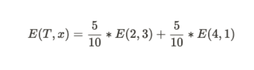
In E(2, 3), p is 2, and q is 3. In E(4, 1), p is 4, and q is 1. Compute the same repeatedly for all the input attributes in the given dataset.
- Using the above two values, calculate the Information Gain or the decrease in entropy by subtracting the entropy of each attribute from the total entropy before the split.
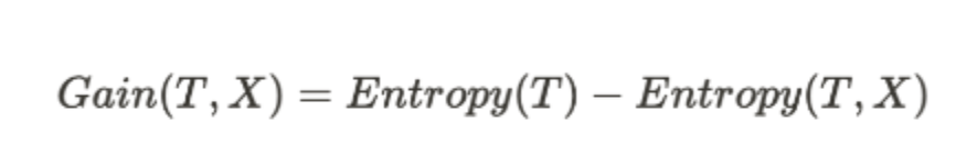
- Choose the attribute that has the highest information gain as the split node.
- Repeat steps 1-4 by dividing the dataset in accordance with the split. This algorithm is run until all the data is classified.
Key Points to Remember:
- A leaf node is a node where entropy is zero, meaning the data is perfectly pure. No further splitting is required at this point.
- Only those branches with entropy greater than zero (i.e., where there is impurity or a mix of classes) need to be split further during the tree-building process.
Chi-Square
The chi-square method works well if the target variables are categorical, like success-failure/high-low. The core idea of the algorithm is to find the statistical significance of the variations that exist between the sub-nodes and the parent node. The mathematical equation that is used to calculate the chi-square is:
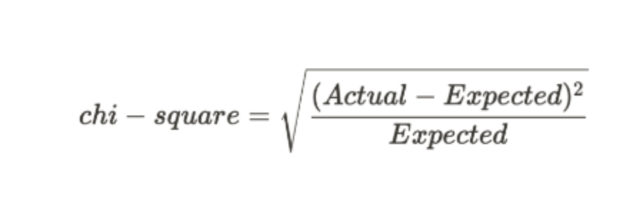
It represents the sum of squares of standardized differences between the target variable’s observed and expected frequencies. One other main advantage of using chi-square is that it can perform multiple splits at a single node, which results in more accuracy and precision.
Applications of Decision Trees
Decision Tree is one of the basic and widely used algorithms in the field of Machine Learning. It’s put into use across different areas in classification and regression modeling. Due to its ability to depict visualized output, one can easily draw insights from the modeling process flow. Here are a few examples where a Decision Tree could be used:
- Business Management
- Customer Relationship Management
- Fraudulent Statement Detection
- Energy Consumption
- Healthcare Management
- Fault Diagnosis
The Hyperparameters
Scikit-learn provides some functionalities or parameters that are to be used with a Decision Tree classifier to enhance the model’s accuracy in accordance with the given data.
- criterion: This parameter is used to measure the quality of the split. The default value for this parameter is set to “Gini”. If you want the measure to be calculated by entropy gain, you can change this parameter to “entropy”.
- splitter: This parameter is used to choose the split at each node. If you want the sub-trees to have the best split, you can set this parameter to “best”. We can also have a random split for which the value “random” is set.
- max-depth: This is an integer parameter through which we can limit the depth of the tree. The default value for this parameter is set to None.
- min_samples_split: This parameter is used to define the minimum number of samples required to split an internal node.
- max_leaf_nodes: The default value of max_leaf_nodes is set to None. This parameter is used to grow a tree with max_leaf_nodes in a best-first fashion.
Code Demo
Step 1: Importing the Modules
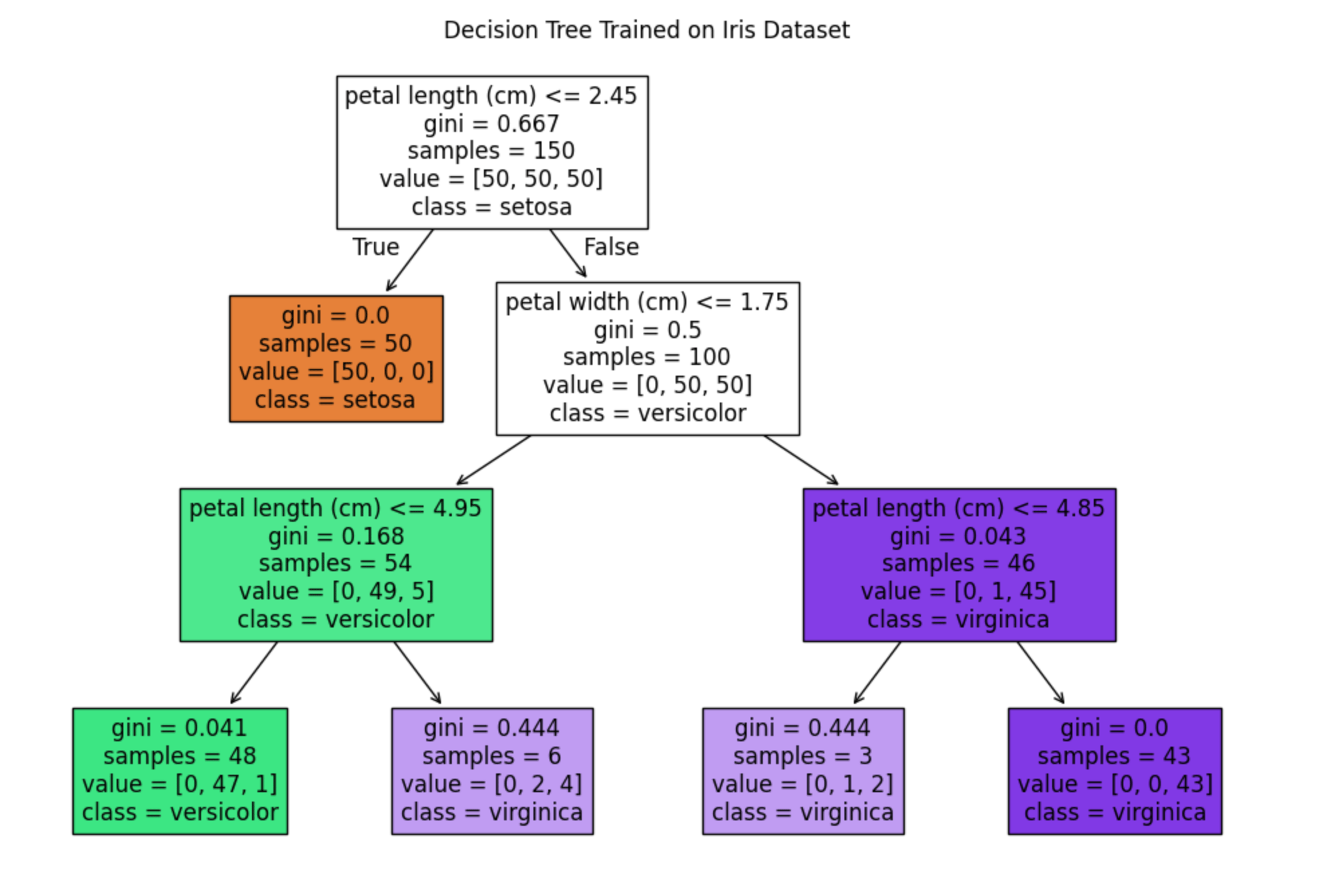
The first and foremost step in building our decision tree model is to import the necessary packages and modules. We import the DecisionTreeClassifier class from the sklearn package. This is an in-built class where the entire decision tree algorithm is coded. In this program, we shall use the iris dataset that can be imported from sklearn.datasets. The pydotplus package is used for visualizing the decision tree. Below is the code snippet,
import pydotplus
from sklearn.tree import DecisionTreeClassifier
from sklearn import datasets
Step 2: Exploring the data
Next, we make our data ready by loading it from the datasets package using the load_iris() method. We assign the data to the iris variable. This iris variable has two keys, one is a data key where all the inputs are present, namely, sepal length, sepal width, petal length, and petal width. In the target key, we have the flower type, which has the values Iris Setosa, Iris Versicolor, and Iris Virginica. We load these in the features and target variables, respectively.
iris = datasets.load_iris()
features = iris.data
target = iris.target

print(features)
print(target)

Output:

[[5.1 3.5 1.4 0.2]
 [4.9 3.  1.4 0.2]
 [4.7 3.2 1.3 0.2]
 [4.6 3.1 1.5 0.2]
 [5.8 4.  1.2 0.2]
 [5.7 4.4 1.5 0.4]
. . . .
. . . .
]
[0 0 0 0 0 0 0 0 0 0 0 0 0 0 0 0 0 0 0 0 0 0 0 0 0 0 0 0 0 0 0 0 0 0 0 0 0 0 0 0 0 0 0 0 0 0 0 0 0 0 1 1 1 1 1 1 1 1 1 1 1 1 1 1 1 1 1 1 1 1 1 1 1 1 1 1 1 1 1 1 1 1 1 1 1 1 1 1 1 1 1 1 1 1 1 1 1 1 1 1 2 2 2 2 2 2 2 2 2 2 2 2 2 2 2 2 2 2 2 2 2 2 2 2 2 2 2 2 2 2 2 2 2 2 2 2 2 2 2 2 2 2 2 2 2 2 2 2 2 2]
This is how our dataset looks.
Step 3: Create a decision tree classifier object
Here, we load the DecisionTreeClassifier in a variable named model, which was imported earlier from the sklearn package.
decisiontree = DecisionTreeClassifier(random_state=0)
Step 5: Fitting the Model
This is the core part of the training process where the decision tree is constructed by making splits in the given data. We train the algorithm with features and target values that are sent as arguments to the fit() method. This method is to fit the data by training the model on features and the target.
model = decisiontree.fit(features, target)
Step 6: Making the Predictions
In this step, we take a sample observation and make a prediction. We create a new list comprising the flower sepal and petal dimensions. Further, we use the predict() method on the trained model to check for the class it belongs to. We can also check the probability (class probability) of the prediction by using the predict_proba method.
observation = [[ 5, 4, 3, 2]] # Predict observation's class
model.predict(observation)
model.predict_proba(observation)

Output:
array([1])
array([[0., 1., 0.]])
Step 7: Dot Data for the predictions
In this step, we export our trained model in DOT format (a graph description language). To achieve that, we use the tree class that can be imported from the sklearn package. On top of that, we use the export_graphviz method with the decision tree, features and the target variables as the parameters.
from sklearn import tree

dot_data = tree.export_graphviz(decisiontree, out_file=None,
feature_names=iris.feature_names,
class_names=iris.target_names
)
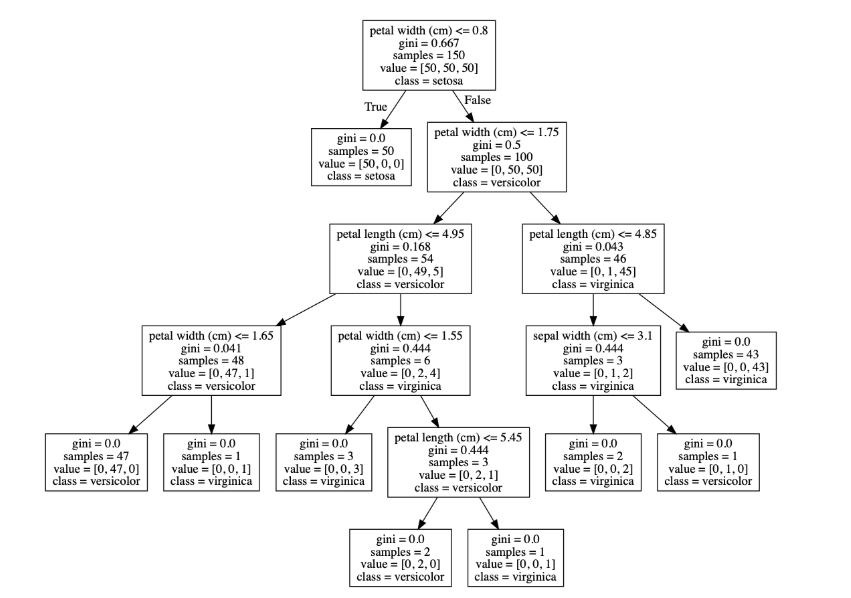
Step 8: Drawing the Graph
In the last step, we visualize the decision tree using an Image class that is to be imported from the IPython.display package.
from IPython.display import Image
graph = pydotplus.graph_from_dot_data(dot_data) # Show graph

Image(graph.create_png())
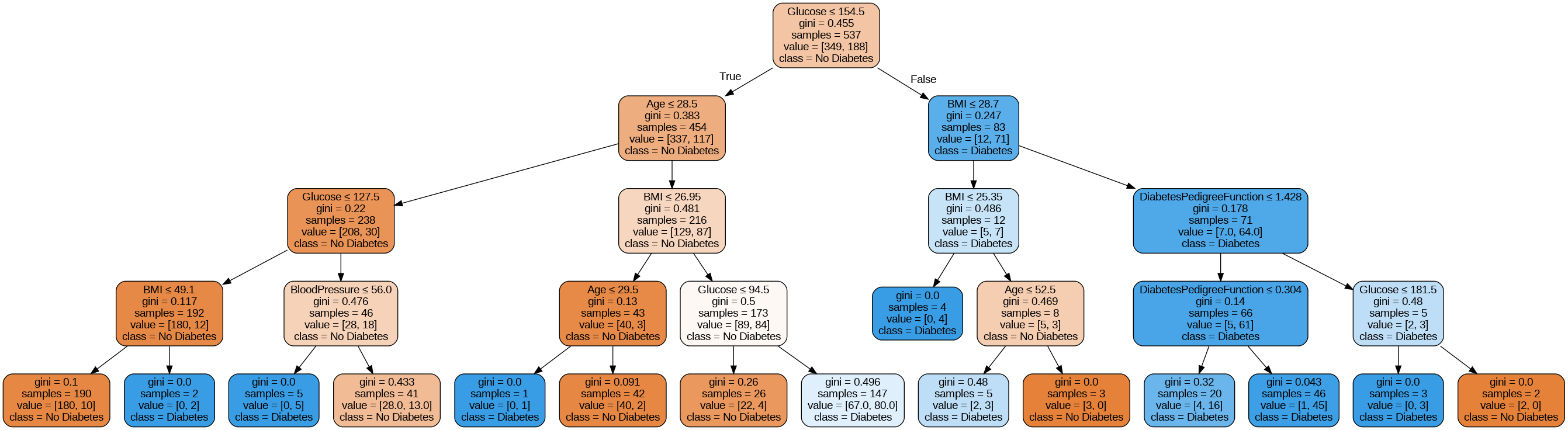
Real-World Application: Predicting Diabetes
We’ll use the popular Pima Indians Diabetes Dataset, a real-world medical dataset where the goal is to predict whether a patient has diabetes based on diagnostic measurements.
Install Dependencies (if not already installed)
pip install scikit-learn graphviz matplotlib pandas seaborn
Step-by-Step Implementation
import pandas as pd
import seaborn as sns
from sklearn.model_selection import train_test_split
from sklearn.tree import DecisionTreeClassifier, export_graphviz, plot_tree
from sklearn.metrics import classification_report, accuracy_score
import matplotlib.pyplot as plt

# Load dataset
df = sns.load_dataset("diabetes") if "diabetes" in sns.get_dataset_names() else pd.read_csv("https://raw.githubusercontent.com/plotly/datasets/master/diabetes.csv")

# Feature matrix and target variable
X = df.drop("Outcome", axis=1)
y = df["Outcome"]

# Train-test split
X_train, X_test, y_train, y_test = train_test_split(X, y, test_size=0.3, random_state=42)

# Build and train decision tree
clf = DecisionTreeClassifier(criterion='gini', max_depth=4, random_state=42)
clf.fit(X_train, y_train)

# Predictions
y_pred = clf.predict(X_test)

# Evaluation
print("Accuracy:", accuracy_score(y_test, y_pred))
print("Classification Report:\n", classification_report(y_test, y_pred))

# Visualize tree using plot_tree
plt.figure(figsize=(20,10))
plot_tree(clf, feature_names=X.columns, class_names=["No Diabetes", "Diabetes"], filled=True, rounded=True)
plt.title("Decision Tree for Diabetes Prediction")
plt.show()
Classification Report:
               precision    recall  f1-score   support

           0       0.85      0.68      0.75       151
           1       0.56      0.78      0.65        80

    accuracy                           0.71       231
   macro avg       0.70      0.73      0.70       231
weighted avg       0.75      0.71      0.72       231
from sklearn.tree import export_graphviz
import graphviz

dot_data = export_graphviz(clf, out_file=None,
                          feature_names=X.columns,
                          class_names=["No Diabetes", "Diabetes"],
                          filled=True, rounded=True,
                          special_characters=True)

graph = graphviz.Source(dot_data)
graph.render("diabetes_tree", format='png', cleanup=False)
graph.view()
Bias-Variance Tradeoff in Decision Trees
When we work with machine learning models, there are often issues when the model behaves extraordinarily well with the training data and poorly when it encounters unseen data. This issue is known as model overfitting. Further, there is also a scenario when the model fits poorly with both the train and the test data, and this is known as model underfitting. Understanding how a model behaves in terms of bias and variance is a necessary step to create a robust and effective ML model.
| Concept | Description |
|---|---|
| Bias | Error due to overly simplistic assumptions in the model. A high-bias tree (e.g., shallow tree) may underfit the data. |
| Variance | Error due to too much complexity in the model. A high-variance tree (e.g., a deep tree) may overfit the training data. |
| Tradeoff | The goal is to find a sweet spot: a depth low enough to generalize well (low variance) but deep enough to capture important patterns (low bias). |
| Solution | Techniques like pruning, setting max_depth, and using ensemble methods like Random Forest can balance the tradeoff. |
Advantages and Disadvantages
There are a few pros and cons that come along with the decision trees. Let’s discuss the advantages first. Decision trees take very little time in processing the data when compared to other algorithms. A few preprocessing steps, like normalization, transformation, and scaling the data, can be skipped. Although there are missing values in the dataset, the performance of the model won’t be affected. A Decision Tree model is intuitive and easy to explain to the technical teams and stakeholders, and can be implemented across several organizations.
Next comes the disadvantages. In decision trees, small changes in the data can cause a large change in the structure of the decision tree, which in turn leads to instability. The training time drastically increases, proportional to the size of the dataset. In some cases, the calculations can become more complex than those of other traditional algorithms.
Conclusion
Decision trees are a great starting point for anyone getting into machine learning. They’re easy to interpret, require minimal data preprocessing, and offer a solid foundation for understanding more advanced techniques. However, they’re not perfect — they can be prone to overfitting, especially when allowed to grow unchecked. That’s why techniques like pruning, setting max depth, or switching to ensemble models are often used in practice. Whether you’re building models for healthcare, finance, e-commerce, or customer analytics, decision trees can help turn your data into meaningful decisions. And if you’re ready to take your machine learning projects to the next level,DigitalOcean offers powerful and cost-effective GPU Droplets that make training models like decision trees faster and more scalable, even for large datasets.
Thanks for learning with the DigitalOcean Community. Check out our offerings for compute, storage, networking, and managed databases.
About the author
With a strong background in data science and over six years of experience, I am passionate about creating in-depth content on technologies. Currently focused on AI, machine learning, and GPU computing, working on topics ranging from deep learning frameworks to optimizing GPU-based workloads.
Still looking for an answer?
This textbox defaults to using Markdown to format your answer.
You can type !ref in this text area to quickly search our full set of tutorials, documentation & marketplace offerings and insert the link!
 This work is licensed under a Creative Commons Attribution-NonCommercial- ShareAlike 4.0 International License.
Become a contributor for community
Get paid to write technical tutorials and select a tech-focused charity to receive a matching donation.

DigitalOcean Documentation
Full documentation for every DigitalOcean product.

Resources for startups and AI-native businesses
The Wave has everything you need to know about building a business, from raising funding to marketing your product.
The developer cloud
Scale up as you grow — whether you're running one virtual machine or ten thousand.

Start building today
From GPU-powered inference and Kubernetes to managed databases and storage, get everything you need to build, scale, and deploy intelligent applications.
