By Alvin Wan and Mark Drake

The author selected Girls Who Code to receive a donation as part of the Write for DOnations program.
Introduction
Reinforcement learning is a subfield within control theory, which concerns controlling systems that change over time and broadly includes applications such as self-driving cars, robotics, and bots for games. Throughout this guide, you will use reinforcement learning to build a bot for Atari video games. This bot is not given access to internal information about the game. Instead, it’s only given access to the game’s rendered display and the reward for that display, meaning that it can only see what a human player would see.
In machine learning, a bot is formally known as an agent. In the case of this tutorial, an agent is a “player” in the system that acts according to a decision-making function, called a policy. The primary goal is to develop strong agents by arming them with strong policies. In other words, our aim is to develop intelligent bots by arming them with strong decision-making capabilities.
You will begin this tutorial by training a basic reinforcement learning agent that takes random actions when playing Space Invaders, the classic Atari arcade game, which will serve as your baseline for comparison. Following this, you will explore several other techniques — including Q-learning, deep Q-learning, and least squares — while building agents that play Space Invaders and Frozen Lake, a simple game environment included in Gym, a reinforcement learning toolkit released by OpenAI. By following this tutorial, you will gain an understanding of the fundamental concepts that govern one’s choice of model complexity in machine learning.
Prerequisites
To complete this tutorial, you will need:
- A server running Ubuntu 18.04, with at least 1GB of RAM. This server should have a non-root user with
sudoprivileges configured, as well as a firewall set up with UFW. You can set this up by following this Initial Server Setup Guide for Ubuntu 18.04. - A Python 3 virtual environment which you can achieve by reading our guide “How To Install Python 3 and Set Up a Programming Environment on an Ubuntu 18.04 Server.”
Alternatively, if you are using a local machine, you can install Python 3 and set up a local programming environment by reading the appropriate tutorial for your operating system via our Python Installation and Setup Series.
Step 1 — Creating the Project and Installing Dependencies
In order to set up the development environment for your bots, you must download the game itself and the libraries needed for computation.
Begin by creating a workspace for this project named AtariBot:
- mkdir ~/AtariBot
Navigate to the new AtariBot directory:
- cd ~/AtariBot
Then create a new virtual environment for the project. You can name this virtual environment anything you’d like; here, we will name it ataribot:
- python3 -m venv ataribot
Activate your environment:
- source ataribot/bin/activate
On Ubuntu, as of version 16.04, OpenCV requires a few more packages to be installed in order to function. These include CMake — an application that manages software build processes — as well as a session manager, miscellaneous extensions, and digital image composition. Run the following command to install these packages:
- sudo apt-get install -y cmake libsm6 libxext6 libxrender-dev libz-dev
NOTE: If you’re following this guide on a local machine running MacOS, the only additional software you need to install is CMake. Install it using Homebrew (which you will have installed if you followed the prerequisite MacOS tutorial) by typing:
- brew install cmake
Next, use pip to install the wheel package, the reference implementation of the wheel packaging standard. A Python library, this package serves as an extension for building wheels and includes a command line tool for working with .whl files:
- python -m pip install wheel
In addition to wheel, you’ll need to install the following packages:
- Gym, a Python library that makes various games available for research, as well as all dependencies for the Atari games. Developed by OpenAI, Gym offers public benchmarks for each of the games so that the performance for various agents and algorithms can be uniformly /evaluated.
- Tensorflow, a deep learning library. This library gives us the ability to run computations more efficiently. Specifically, it does this by building mathematical functions using Tensorflow’s abstractions that run exclusively on your GPU.
- OpenCV, the computer vision library mentioned previously.
- SciPy, a scientific computing library that offers efficient optimization algorithms.
- NumPy, a linear algebra library.
Install each of these packages with the following command. Note that this command specifies which version of each package to install:
- python -m pip install gym==0.9.5 tensorflow==1.5.0 tensorpack==0.8.0 numpy==1.14.0 scipy==1.1.0 opencv-python==3.4.1.15
Following this, use pip once more to install Gym’s Atari environments, which includes a variety of Atari video games, including Space Invaders:
- python -m pip install gym[atari]
If your installation of the gym[atari] package was successful, your output will end with the following:
OutputInstalling collected packages: atari-py, Pillow, PyOpenGL
Successfully installed Pillow-5.4.1 PyOpenGL-3.1.0 atari-py-0.1.7
With these dependencies installed, you’re ready to move on and build an agent that plays randomly to serve as your baseline for comparison.
Step 2 — Creating a Baseline Random Agent with Gym
Now that the required software is on your server, you will set up an agent that will play a simplified version of the classic Atari game, Space Invaders. For any experiment, it is necessary to obtain a baseline to help you understand how well your model performs. Because this agent takes random actions at each frame, we’ll refer to it as our random, baseline agent. In this case, you will compare against this baseline agent to understand how well your agents perform in later steps.
With Gym, you maintain your own game loop. This means that you handle every step of the game’s execution: at every time step, you give the gym a new action and ask gym for the game state. In this tutorial, the game state is the game’s appearance at a given time step, and is precisely what you would see if you were playing the game.
Using your preferred text editor, create a Python file named bot_2_random.py. Here, we’ll use nano:
- nano bot_2_random.py
Note: Throughout this guide, the bots’ names are aligned with the Step number in which they appear, rather than the order in which they appear. Hence, this bot is named bot_2_random.py rather than bot_1_random.py.
Start this script by adding the following highlighted lines. These lines include a comment block that explains what this script will do and two import statements that will import the packages this script will ultimately need in order to function:
"""
Bot 2 -- Make a random, baseline agent for the SpaceInvaders game.
"""

import gym
import random
Add a main function. In this function, create the game environment — SpaceInvaders-v0 — and then initialize the game using env.reset:
. . .
import gym
import random

def main():
    env = gym.make('SpaceInvaders-v0')
    env.reset()
Next, add an env.step function. This function can return the following kinds of values:
state: The new state of the game, after applying the provided action.reward: The increase in score that the state incurs. By way of example, this could be when a bullet has destroyed an alien, and the score increases by 50 points. Then,reward = 50. In playing any score-based game, the player’s goal is to maximize the score. This is synonymous with maximizing the total reward.done: Whether or not the episode has ended, which usually occurs when a player has lost all lives.info: Extraneous information that you’ll put aside for now.
You will use reward to count your total reward. You’ll also use done to determine when the player dies, which will be when done returns True.
Add the following game loop, which instructs the game to loop until the player dies:
. . .
def main():
    env = gym.make('SpaceInvaders-v0')
    env.reset()

    episode_reward = 0
    while True:
        action = env.action_space.sample()
        _, reward, done, _ = env.step(action)
        episode_reward += reward
        if done:
            print('Reward: %s' % episode_reward)
            break
Finally, run the main function. Include a __name__ check to ensure that main only runs when you invoke it directly with python bot_2_random.py. If you do not add the if check, main will always be triggered when the Python file is executed, even when you import the file. Consequently, it’s a good practice to place the code in a main function, executed only when __name__ == '__main__'.
. . .
def main():
    . . .
    if done:
        print('Reward %s' % episode_reward)
        break

if __name__ == '__main__':
    main()
Save the file and exit the editor. If you’re using nano, do so by pressing CTRL+X, Y, then ENTER. Then, run your script by typing:
- python bot_2_random.py
Your program will output a number, akin to the following. Note that each time you run the file you will get a different result:
OutputMaking new env: SpaceInvaders-v0
Reward: 210.0
These random results present an issue. In order to produce work that other researchers and practitioners can benefit from, your results and trials must be reproducible. To correct this, reopen the script file:
- nano bot_2_random.py
After import random, add random.seed(0). After env = gym.make('SpaceInvaders-v0'), add env.seed(0). Together, these lines “seed” the environment with a consistent starting point, ensuring that the results will always be reproducible. Your final file will match the following, exactly:
"""
Bot 2 -- Make a random, baseline agent for the SpaceInvaders game.
"""

import gym
import random
random.seed(0)


def main():
    env = gym.make('SpaceInvaders-v0')
    env.seed(0)

    env.reset()
    episode_reward = 0
    while True:
        action = env.action_space.sample()
        _, reward, done, _ = env.step(action)
        episode_reward += reward
        if done:
            print('Reward: %s' % episode_reward)
            break


if __name__ == '__main__':
    main()
Save the file and close your editor, then run the script by typing the following in your terminal:
- python bot_2_random.py
This will output the following reward, exactly:
OutputMaking new env: SpaceInvaders-v0
Reward: 555.0
This is your very first bot, although it’s rather unintelligent since it doesn’t account for the surrounding environment when it makes decisions. For a more reliable estimate of your bot’s performance, you could have the agent run for multiple episodes at a time, reporting rewards averaged across multiple episodes. To configure this, first reopen the file:
- nano bot_2_random.py
After random.seed(0), add the following highlighted line which tells the agent to play the game for 10 episodes:
. . .
random.seed(0)

num_episodes = 10
. . .
Right after env.seed(0), start a new list of rewards:
. . .
    env.seed(0)
    rewards = []
. . .
Nest all code from env.reset() to the end of main() in a for loop, iterating num_episodes times. Make sure to indent each line from env.reset() to break by four spaces:
. . .
def main():
    env = gym.make('SpaceInvaders-v0')
    env.seed(0)
    rewards = []

    for _ in range(num_episodes):
        env.reset()
        episode_reward = 0

        while True:
            ...
Right before break, currently the last line of the main game loop, add the current episode’s reward to the list of all rewards:
. . .
        if done:
            print('Reward: %s' % episode_reward)
            rewards.append(episode_reward)
            break
. . .
At the end of the main function, report the average reward:
. . .
def main():
    ...
            print('Reward: %s' % episode_reward)
            break
    print('Average reward: %.2f' % (sum(rewards) / len(rewards)))
    . . .
Your file will now align with the following. Please note that the following code block includes a few comments to clarify key parts of the script:
"""
Bot 2 -- Make a random, baseline agent for the SpaceInvaders game.
"""

import gym
import random
random.seed(0)  # make results reproducible

num_episodes = 10


def main():
    env = gym.make('SpaceInvaders-v0')  # create the game
    env.seed(0)  # make results reproducible
    rewards = []

    for _ in range(num_episodes):
        env.reset()
        episode_reward = 0
        while True:
            action = env.action_space.sample()
            _, reward, done, _ = env.step(action)  # random action
            episode_reward += reward
            if done:
                print('Reward: %d' % episode_reward)
                rewards.append(episode_reward)
                break
    print('Average reward: %.2f' % (sum(rewards) / len(rewards)))


if __name__ == '__main__':
    main()
Save the file, exit the editor, and run the script:
- python bot_2_random.py
This will print the following average reward, exactly:
OutputMaking new env: SpaceInvaders-v0
. . .
Average reward: 163.50
We now have a more reliable estimate of the baseline score to beat. To create a superior agent, though, you will need to understand the framework for reinforcement learning. How can one make the abstract notion of “decision-making” more concrete?
Understanding Reinforcement Learning
In any game, the player’s goal is to maximize their score. In this guide, the player’s score is referred to as its reward. To maximize their reward, the player must be able to refine its decision-making abilities. Formally, a decision is the process of looking at the game, or observing the game’s state, and picking an action. Our decision-making function is called a policy; a policy accepts a state as input and “decides” on an action:
policy: state -> action
To build such a function, we will start with a specific set of algorithms in reinforcement learning called Q-learning algorithms. To illustrate these, consider the initial state of a game, which we’ll call state0: your spaceship and the aliens are all in their starting positions. Then, assume we have access to a magical “Q-table” which tells us how much reward each action will earn:
| state | action | reward |
|---|---|---|
| state0 | shoot | 10 |
| state0 | right | 3 |
| state0 | left | 3 |
The shoot action will maximize your reward, as it results in the reward with the highest value: 10. As you can see, a Q-table provides a straightforward way to make decisions, based on the observed state:
policy: state -> look at Q-table, pick action with greatest reward
However, most games have too many states to list in a table. In such cases, the Q-learning agent learns a Q-function instead of a Q-table. We use this Q-function similarly to how we used the Q-table previously. Rewriting the table entries as functions gives us the following:
Q(state0, shoot) = 10
Q(state0, right) = 3
Q(state0, left) = 3
Given a particular state, it’s easy for us to make a decision: we simply look at each possible action and its reward, then take the action that corresponds with the highest expected reward. Reformulating the earlier policy more formally, we have:
policy: state -> argmax_{action} Q(state, action)
This satisfies the requirements of a decision-making function: given a state in the game, it decides on an action. However, this solution depends on knowing Q(state, action) for every state and action. To estimate Q(state, action), consider the following:
- Given many observations of an agent’s states, actions, and rewards, one can obtain an estimate of the reward for every state and action by taking a running average.
- Space Invaders is a game with delayed rewards: the player is rewarded when the alien is blown up and not when the player shoots. However, the player taking an action by shooting is the true impetus for the reward. Somehow, the Q-function must assign
(state0, shoot)a positive reward.
These two insights are codified in the following equations:
Q(state, action) = (1 - learning_rate) * Q(state, action) + learning_rate * Q_target
Q_target = reward + discount_factor * max_{action'} Q(state', action')
These equations use the following definitions:
state: the state at current time stepaction: the action taken at current time stepreward: the reward for current time stepstate': the new state for next time step, given that we took actionaaction': all possible actionslearning_rate: the learning ratediscount_factor: the discount factor, how much reward “degrades” as we propagate it
For a complete explanation of these two equations, see this article on Understanding Q-Learning.
With this understanding of reinforcement learning in mind, all that remains is to actually run the game and obtain these Q-value estimates for a new policy.
Step 3 — Creating a Simple Q-learning Agent for Frozen Lake
Now that you have a baseline agent, you can begin creating new agents and compare them against the original. In this step, you will create an agent that uses Q-learning, a reinforcement learning technique used to teach an agent which action to take given a certain state. This agent will play a new game, FrozenLake. The setup for this game is described as follows on the Gym website:
Winter is here. You and your friends were tossing around a frisbee at the park when you made a wild throw that left the frisbee out in the middle of the lake. The water is mostly frozen, but there are a few holes where the ice has melted. If you step into one of those holes, you’ll fall into the freezing water. At this time, there’s an international frisbee shortage, so it’s absolutely imperative that you navigate across the lake and retrieve the disc. However, the ice is slippery, so you won’t always move in the direction you intend.
The surface is described using a grid like the following:
SFFF       (S: starting point, safe)
FHFH       (F: frozen surface, safe)
FFFH       (H: hole, fall to your doom)
HFFG       (G: goal, where the frisbee is located)
The player starts at the top left, denoted by S, and works its way to the goal at the bottom right, denoted by G. The available actions are right, left, up, and down, and reaching the goal results in a score of 1. There are a number of holes, denoted H, and falling into one immediately results in a score of 0.
In this section, you will implement a simple Q-learning agent. Using what you’ve learned previously, you will create an agent that trades off between exploration and exploitation. In this context, exploration means the agent acts randomly, and exploitation means it uses its Q-values to choose what it believes to be the optimal action. You will also create a table to hold the Q-values, updating it incrementally as the agent acts and learns.
Make a copy of your script from Step 2:
- cp bot_2_random.py bot_3_q_table.py
Then open up this new file for editing:
- nano bot_3_q_table.py
Begin by updating the comment at the top of the file that describes the script’s purpose. Because this is only a comment, this change isn’t necessary for the script to function properly, but it can be helpful for keeping track of what the script does:
"""
Bot 3 -- Build simple q-learning agent for FrozenLake
"""

. . .
Before you make functional modifications to the script, you will need to import numpy for its linear algebra utilities. Right underneath import gym, add the highlighted line:
"""
Bot 3 -- Build simple q-learning agent for FrozenLake
"""

import gym
import numpy as np
import random
random.seed(0)  # make results reproducible
. . .
Underneath random.seed(0), add a seed for numpy:
. . .
import random
random.seed(0)  # make results reproducible
np.random.seed(0)
. . .
Next, make the game states accessible. Update the env.reset() line to say the following, which stores the initial state of the game in the variable state:
. . .
    for _ in range(num_episodes):
        state = env.reset()
        . . .
Update the env.step(...) line to say the following, which stores the next state, state2. You will need both the current state and the next one — state2 — to update the Q-function.
        . . .
        while True:
            action = env.action_space.sample()
            state2, reward, done, _ = env.step(action)
            . . .
After episode_reward += reward, add a line updating the variable state. This keeps the variable state updated for the next iteration, as you will expect state to reflect the current state:
. . .
        while True:
            . . .
            episode_reward += reward
            state = state2
            if done:
                . . .
In the if done block, delete the print statement which prints the reward for each episode. Instead, you’ll output the average reward over many episodes. The if done block will then look like this:
            . . .
            if done:
                rewards.append(episode_reward)
                break
                . . .
After these modifications your game loop will match the following:
. . .
    for _ in range(num_episodes):
        state = env.reset()
        episode_reward = 0
        while True:
            action = env.action_space.sample()
            state2, reward, done, _ = env.step(action)
            episode_reward += reward
            state = state2
            if done:
                rewards.append(episode_reward))
                break
                . . .
Next, add the ability for the agent to trade off between exploration and exploitation. Right before your main game loop (which starts with for...), create the Q-value table:
. . .
    Q = np.zeros((env.observation_space.n, env.action_space.n))
    for _ in range(num_episodes):
      . . .
Then, rewrite the for loop to expose the episode number:
. . .
    Q = np.zeros((env.observation_space.n, env.action_space.n))
    for episode in range(1, num_episodes + 1):
      . . .
Inside the while True: inner game loop, create noise. Noise, or meaningless, random data, is sometimes introduced when training deep neural networks because it can improve both the performance and the accuracy of the model. Note that the higher the noise, the less the values in Q[state, :] matter. As a result, the higher the noise, the more likely that the agent acts independently of its knowledge of the game. In other words, higher noise encourages the agent to explore random actions:
        . . .
        while True:
            noise = np.random.random((1, env.action_space.n)) / (episode**2.)
            action = env.action_space.sample()
            . . .
Note that as episodes increases, the amount of noise decreases quadratically: as time goes on, the agent explores less and less because it can trust its own assessment of the game’s reward and begin to exploit its knowledge.
Update the action line to have your agent pick actions according to the Q-value table, with some exploration built in:
            . . .
            noise = np.random.random((1, env.action_space.n)) / (episode**2.)
            action = np.argmax(Q[state, :] + noise)
            state2, reward, done, _ = env.step(action)
            . . .
Your main game loop will then match the following:
. . .
    Q = np.zeros((env.observation_space.n, env.action_space.n))
    for episode in range(1, num_episodes + 1):
        state = env.reset()
        episode_reward = 0
        while True:
            noise = np.random.random((1, env.action_space.n)) / (episode**2.)
            action = np.argmax(Q[state, :] + noise)
            state2, reward, done, _ = env.step(action)
            episode_reward += reward
            state = state2
            if done:
                rewards.append(episode_reward)
                break
                . . .
Next, you will update your Q-value table using the Bellman update equation, an equation widely used in machine learning to find the optimal policy within a given environment.
The Bellman equation incorporates two ideas that are highly relevant to this project. First, taking a particular action from a particular state many times will result in a good estimate for the Q-value associated with that state and action. To this end, you will increase the number of episodes this bot must play through in order to return a stronger Q-value estimate. Second, rewards must propagate through time, so that the original action is assigned a non-zero reward. This idea is clearest in games with delayed rewards; for example, in Space Invaders, the player is rewarded when the alien is blown up and not when the player shoots. However, the player shooting is the true impetus for a reward. Likewise, the Q-function must assign (state0, shoot) a positive reward.
First, update num_episodes to equal 4000:
. . .
np.random.seed(0)

num_episodes = 4000
. . .
Then, add the necessary hyperparameters to the top of the file in the form of two more variables:
. . .
num_episodes = 4000
discount_factor = 0.8
learning_rate = 0.9
. . .
Compute the new target Q-value, right after the line containing env.step(...):
            . . .
            state2, reward, done, _ = env.step(action)
            Qtarget = reward + discount_factor * np.max(Q[state2, :])
            episode_reward += reward
            . . .
On the line directly after Qtarget, update the Q-value table using a weighted average of the old and new Q-values:
            . . .
            Qtarget = reward + discount_factor * np.max(Q[state2, :])
            Q[state, action] = (1-learning_rate) * Q[state, action] + learning_rate * Qtarget
            episode_reward += reward
            . . .
Check that your main game loop now matches the following:
. . .
    Q = np.zeros((env.observation_space.n, env.action_space.n))
    for episode in range(1, num_episodes + 1):
        state = env.reset()
        episode_reward = 0
        while True:
            noise = np.random.random((1, env.action_space.n)) / (episode**2.)
            action = np.argmax(Q[state, :] + noise)
            state2, reward, done, _ = env.step(action)
            Qtarget = reward + discount_factor * np.max(Q[state2, :])
            Q[state, action] = (1-learning_rate) * Q[state, action] + learning_rate * Qtarget
            episode_reward += reward
            state = state2
            if done:
                rewards.append(episode_reward)
                break
                . . .
Our logic for training the agent is now complete. All that’s left is to add reporting mechanisms.
Even though Python does not enforce strict type checking, add types to your function declarations for cleanliness. At the top of the file, before the first line reading import gym, import the List type:
. . .
from typing import List
import gym
. . .
Right after learning_rate = 0.9, outside of the main function, declare the interval and format for reports:
. . .
learning_rate = 0.9
report_interval = 500
report = '100-ep Average: %.2f . Best 100-ep Average: %.2f . Average: %.2f ' \
         '(Episode %d)'

def main():
  . . .
Before the main function, add a new function that will populate this report string, using the list of all rewards:
. . .
report = '100-ep Average: %.2f . Best 100-ep Average: %.2f . Average: %.2f ' \
         '(Episode %d)'

def print_report(rewards: List, episode: int):
    """Print rewards report for current episode
    - Average for last 100 episodes
    - Best 100-episode average across all time
    - Average for all episodes across time
    """
    print(report % (
        np.mean(rewards[-100:]),
        max([np.mean(rewards[i:i+100]) for i in range(len(rewards) - 100)]),
        np.mean(rewards),
        episode))


def main():
  . . .
Change the game to FrozenLake instead of SpaceInvaders:
. . .
def main():
    env = gym.make('FrozenLake-v0')  # create the game
    . . .
After rewards.append(...), print the average reward over the last 100 episodes and print the average reward across all episodes:
            . . .
            if done:
                rewards.append(episode_reward)
                if episode % report_interval == 0:
                    print_report(rewards, episode)
                . . .
At the end of the main() function, report both averages once more. Do this by replacing the line that reads print('Average reward: %.2f' % (sum(rewards) / len(rewards))) with the following highlighted line:
. . .
def main():
    ...
                break
    print_report(rewards, -1)
. . .
Finally, you have completed your Q-learning agent. Check that your script aligns with the following:
"""
Bot 3 -- Build simple q-learning agent for FrozenLake
"""

from typing import List
import gym
import numpy as np
import random
random.seed(0)  # make results reproducible
np.random.seed(0)  # make results reproducible

num_episodes = 4000
discount_factor = 0.8
learning_rate = 0.9
report_interval = 500
report = '100-ep Average: %.2f . Best 100-ep Average: %.2f . Average: %.2f ' \
         '(Episode %d)'


def print_report(rewards: List, episode: int):
    """Print rewards report for current episode
    - Average for last 100 episodes
    - Best 100-episode average across all time
    - Average for all episodes across time
    """
    print(report % (
        np.mean(rewards[-100:]),
        max([np.mean(rewards[i:i+100]) for i in range(len(rewards) - 100)]),
        np.mean(rewards),
        episode))


def main():
    env = gym.make('FrozenLake-v0')  # create the game
    env.seed(0)  # make results reproducible
    rewards = []

    Q = np.zeros((env.observation_space.n, env.action_space.n))
    for episode in range(1, num_episodes + 1):
        state = env.reset()
        episode_reward = 0
        while True:
            noise = np.random.random((1, env.action_space.n)) / (episode**2.)
            action = np.argmax(Q[state, :] + noise)
            state2, reward, done, _ = env.step(action)
            Qtarget = reward + discount_factor * np.max(Q[state2, :])
            Q[state, action] = (1-learning_rate) * Q[state, action] + learning_rate * Qtarget
            episode_reward += reward
            state = state2
            if done:
                rewards.append(episode_reward)
                if episode % report_interval == 0:
                    print_report(rewards, episode)
                break
    print_report(rewards, -1)

if __name__ == '__main__':
    main()
Save the file, exit your editor, and run the script:
- python bot_3_q_table.py
Your output will match the following:
Output100-ep Average: 0.11 . Best 100-ep Average: 0.12 . Average: 0.03 (Episode 500)
100-ep Average: 0.25 . Best 100-ep Average: 0.24 . Average: 0.09 (Episode 1000)
100-ep Average: 0.39 . Best 100-ep Average: 0.48 . Average: 0.19 (Episode 1500)
100-ep Average: 0.43 . Best 100-ep Average: 0.55 . Average: 0.25 (Episode 2000)
100-ep Average: 0.44 . Best 100-ep Average: 0.55 . Average: 0.29 (Episode 2500)
100-ep Average: 0.64 . Best 100-ep Average: 0.68 . Average: 0.32 (Episode 3000)
100-ep Average: 0.63 . Best 100-ep Average: 0.71 . Average: 0.36 (Episode 3500)
100-ep Average: 0.56 . Best 100-ep Average: 0.78 . Average: 0.40 (Episode 4000)
100-ep Average: 0.56 . Best 100-ep Average: 0.78 . Average: 0.40 (Episode -1)
You now have your first non-trivial bot for games, but let’s put this average reward of 0.78 into perspective. According to the Gym FrozenLake page, “solving” the game means attaining a 100-episode average of 0.78. Informally, “solving” means “plays the game very well”. While not in record time, the Q-table agent is able to solve FrozenLake in 4000 episodes.
However, the game may be more complex. Here, you used a table to store all of the 144 possible states, but consider tic tac toe in which there are 19,683 possible states. Likewise, consider Space Invaders where there are too many possible states to count. A Q-table is not sustainable as games grow increasingly complex. For this reason, you need some way to approximate the Q-table. As you continue experimenting in the next step, you will design a function that can accept states and actions as inputs and output a Q-value.
Step 4 — Building a Deep Q-learning Agent for Frozen Lake
In reinforcement learning, the neural network effectively predicts the value of Q based on the state and action inputs, using a table to store all the possible values, but this becomes unstable in complex games. Deep reinforcement learning instead uses a neural network to approximate the Q-function. For more details, see Understanding Deep Q-Learning.
To get accustomed to Tensorflow, a deep learning library you installed in Step 1, you will reimplement all of the logic used so far with Tensorflow’s abstractions and you’ll use a neural network to approximate your Q-function. However, your neural network will be extremely simple: your output Q(s) is a matrix W multiplied by your input s. This is known as a neural network with one fully-connected layer:
Q(s) = Ws
To reiterate, the goal is to reimplement all of the logic from the bots we’ve already built using Tensorflow’s abstractions. This will make your operations more efficient, as Tensorflow can then perform all computation on the GPU.
Begin by duplicating your Q-table script from Step 3:
- cp bot_3_q_table.py bot_4_q_network.py
Then open the new file with nano or your preferred text editor:
- nano bot_4_q_network.py
First, update the comment at the top of the file:
"""
Bot 4 -- Use Q-learning network to train bot
"""

. . .
Next, import the Tensorflow package by adding an import directive right below import random. Additionally, add tf.set_radon_seed(0) right below np.random.seed(0). This will ensure that the results of this script will be repeatable across all sessions:
. . .
import random
import tensorflow as tf
random.seed(0)
np.random.seed(0)
tf.set_random_seed(0)
. . .
Redefine your hyperparameters at the top of the file to match the following and add a function called exploration_probability, which will return the probability of exploration at each step. Remember that, in this context, “exploration” means taking a random action, as opposed to taking the action recommended by the Q-value estimates:
. . .
num_episodes = 4000
discount_factor = 0.99
learning_rate = 0.15
report_interval = 500
exploration_probability = lambda episode: 50. / (episode + 10)
report = '100-ep Average: %.2f . Best 100-ep Average: %.2f . Average: %.2f ' \
         '(Episode %d)'
. . .
Next, you will add a one-hot encoding function. In short, one-hot encoding is a process through which variables are converted into a form that helps machine learning algorithms make better predictions. If you’d like to learn more about one-hot encoding, you can check out Adversarial Examples in Computer Vision: How to Build then Fool an Emotion-Based Dog Filter.
Directly beneath report = ..., add a one_hot function:
. . .
report = '100-ep Average: %.2f . Best 100-ep Average: %.2f . Average: %.2f ' \
         '(Episode %d)'

def one_hot(i: int, n: int) -> np.array:
    """Implements one-hot encoding by selecting the ith standard basis vector"""
    return np.identity(n)[i].reshape((1, -1))

def print_report(rewards: List, episode: int):
. . .
Next, you will rewrite your algorithm logic using Tensorflow’s abstractions. Before doing that, though, you’ll need to first create placeholders for your data.
In your main function, directly beneath rewards=[], insert the following highlighted content. Here, you define placeholders for your observation at time t (as obs_t_ph) and time t+1 (as obs_tp1_ph), as well as placeholders for your action, reward, and Q target:
. . .
def main():
    env = gym.make('FrozenLake-v0')  # create the game
    env.seed(0)  # make results reproducible
    rewards = []

    # 1. Setup placeholders
    n_obs, n_actions = env.observation_space.n, env.action_space.n
    obs_t_ph = tf.placeholder(shape=[1, n_obs], dtype=tf.float32)
    obs_tp1_ph = tf.placeholder(shape=[1, n_obs], dtype=tf.float32)
    act_ph = tf.placeholder(tf.int32, shape=())
    rew_ph = tf.placeholder(shape=(), dtype=tf.float32)
    q_target_ph = tf.placeholder(shape=[1, n_actions], dtype=tf.float32)

    Q = np.zeros((env.observation_space.n, env.action_space.n))
    for episode in range(1, num_episodes + 1):
        . . .
Directly beneath the line beginning with q_target_ph =, insert the following highlighted lines. This code starts your computation by computing Q(s, a) for all a to make q_current and Q(s’, a’) for all a’ to make q_target:
    . . .
    rew_ph = tf.placeholder(shape=(), dtype=tf.float32)
    q_target_ph = tf.placeholder(shape=[1, n_actions], dtype=tf.float32)

    # 2. Setup computation graph
    W = tf.Variable(tf.random_uniform([n_obs, n_actions], 0, 0.01))
    q_current = tf.matmul(obs_t_ph, W)
    q_target = tf.matmul(obs_tp1_ph, W)

    Q = np.zeros((env.observation_space.n, env.action_space.n))
    for episode in range(1, num_episodes + 1):
        . . .
Again directly beneath the last line you added, insert the following higlighted code. The first two lines are equivalent to the line added in Step 3 that computes Qtarget, where Qtarget = reward + discount_factor * np.max(Q[state2, :]). The next two lines set up your loss, while the last line computes the action that maximizes your Q-value:
    . . .
    q_current = tf.matmul(obs_t_ph, W)
    q_target = tf.matmul(obs_tp1_ph, W)

    q_target_max = tf.reduce_max(q_target_ph, axis=1)
    q_target_sa = rew_ph + discount_factor * q_target_max
    q_current_sa = q_current[0, act_ph]
    error = tf.reduce_sum(tf.square(q_target_sa - q_current_sa))
    pred_act_ph = tf.argmax(q_current, 1)

    Q = np.zeros((env.observation_space.n, env.action_space.n))
    for episode in range(1, num_episodes + 1):
        . . .
After setting up your algorithm and the loss function, define your optimizer:
    . . .
    error = tf.reduce_sum(tf.square(q_target_sa - q_current_sa))
    pred_act_ph = tf.argmax(q_current, 1)

    # 3. Setup optimization
    trainer = tf.train.GradientDescentOptimizer(learning_rate=learning_rate)
    update_model = trainer.minimize(error)

    Q = np.zeros((env.observation_space.n, env.action_space.n))
    for episode in range(1, num_episodes + 1):
        . . .
Next, set up the body of the game loop. To do this, pass data to the Tensorflow placeholders and Tensorflow’s abstractions will handle the computation on the GPU, returning the result of the algorithm.
Start by deleting the old Q-table and logic. Specifically, delete the lines that define Q (right before the for loop), noise (in the while loop), action, Qtarget, and Q[state, action]. Rename state to obs_t and state2 to obs_tp1 to align with the Tensorflow placeholders you set previously. When finished, your for loop will match the following:
    . . .
    # 3. Setup optimization
    trainer = tf.train.GradientDescentOptimizer(learning_rate=learning_rate)
    update_model = trainer.minimize(error)

    for episode in range(1, num_episodes + 1):
        obs_t = env.reset()
        episode_reward = 0
        while True:

            obs_tp1, reward, done, _ = env.step(action)

            episode_reward += reward
            obs_t = obs_tp1
            if done:
                ...
Directly above the for loop, add the following two highlighted lines. These lines initialize a Tensorflow session which in turn manages the resources needed to run operations on the GPU. The second line initializes all the variables in your computation graph; for example, initializing weights to 0 before updating them. Additionally, you will nest the for loop within the with statement, so indent the entire for loop by four spaces:
    . . .
    trainer = tf.train.GradientDescentOptimizer(learning_rate=learning_rate)
        update_model = trainer.minimize(error)

    with tf.Session() as session:
        session.run(tf.global_variables_initializer())

        for episode in range(1, num_episodes + 1):
            obs_t = env.reset()
            ...
Before the line reading obs_tp1, reward, done, _ = env.step(action), insert the following lines to compute the action. This code evaluates the corresponding placeholder and replaces the action with a random action with some probability:
            . . .
            while True:
                # 4. Take step using best action or random action
                obs_t_oh = one_hot(obs_t, n_obs)
                action = session.run(pred_act_ph, feed_dict={obs_t_ph: obs_t_oh})[0]
                if np.random.rand(1) < exploration_probability(episode):
                    action = env.action_space.sample()
                . . .
After the line containing env.step(action), insert the following to train the neural network in estimating your Q-value function:
                . . .
                obs_tp1, reward, done, _ = env.step(action)

                # 5. Train model
                obs_tp1_oh = one_hot(obs_tp1, n_obs)
                q_target_val = session.run(q_target, feed_dict={obs_tp1_ph: obs_tp1_oh})
                session.run(update_model, feed_dict={
                    obs_t_ph: obs_t_oh,
                    rew_ph: reward,
                    q_target_ph: q_target_val,
                    act_ph: action
                })
                episode_reward += reward
                . . .
Your final file will match this file hosted on GitHub. Save the file, exit your editor, and run the script:
- python bot_4_q_network.py
Your output will end with the following, exactly:
Output100-ep Average: 0.11 . Best 100-ep Average: 0.11 . Average: 0.05 (Episode 500)
100-ep Average: 0.41 . Best 100-ep Average: 0.54 . Average: 0.19 (Episode 1000)
100-ep Average: 0.56 . Best 100-ep Average: 0.73 . Average: 0.31 (Episode 1500)
100-ep Average: 0.57 . Best 100-ep Average: 0.73 . Average: 0.36 (Episode 2000)
100-ep Average: 0.65 . Best 100-ep Average: 0.73 . Average: 0.41 (Episode 2500)
100-ep Average: 0.65 . Best 100-ep Average: 0.73 . Average: 0.43 (Episode 3000)
100-ep Average: 0.69 . Best 100-ep Average: 0.73 . Average: 0.46 (Episode 3500)
100-ep Average: 0.77 . Best 100-ep Average: 0.79 . Average: 0.48 (Episode 4000)
100-ep Average: 0.77 . Best 100-ep Average: 0.79 . Average: 0.48 (Episode -1)
You’ve now trained your very first deep Q-learning agent. For a game as simple as FrozenLake, your deep Q-learning agent required 4000 episodes to train. Imagine if the game were far more complex. How many training samples would that require to train? As it turns out, the agent could require millions of samples. The number of samples required is referred to as sample complexity, a concept explored further in the next section.
Understanding Bias-Variance Tradeoffs
Generally speaking, sample complexity is at odds with model complexity in machine learning:
- Model complexity: One wants a sufficiently complex model to solve their problem. For example, a model as simple as a line is not sufficiently complex to predict a car’s trajectory.
- Sample complexity: One would like a model that does not require many samples. This could be because they have a limited access to labeled data, an insufficient amount of computing power, limited memory, etc.
Say we have two models, one simple and one extremely complex. For both models to attain the same performance, bias-variance tells us that the extremely complex model will need exponentially more samples to train. Case in point: your neural network-based Q-learning agent required 4000 episodes to solve FrozenLake. Adding a second layer to the neural network agent quadruples the number of necessary training episodes. With increasingly complex neural networks, this divide only grows. To maintain the same error rate, increasing model complexity increases the sample complexity exponentially. Likewise, decreasing sample complexity decreases model complexity. Thus, we cannot maximize model complexity and minimize sample complexity to our heart’s desire.
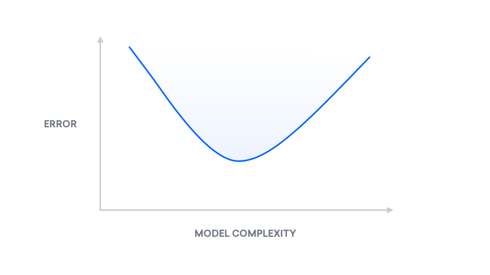
We can, however, leverage our knowledge of this tradeoff. For a visual interpretation of the mathematics behind the bias-variance decomposition, see Understanding the Bias-Variance Tradeoff. At a high level, the bias-variance decomposition is a breakdown of “true error” into two components: bias and variance. We refer to “true error” as mean squared error (MSE), which is the expected difference between our predicted labels and the true labels. The following is a plot showing the change of “true error” as model complexity increases:
Step 5 — Building a Least Squares Agent for Frozen Lake
The least squares method, also known as linear regression, is a means of regression analysis used widely in the fields of mathematics and data science. In machine learning, it’s often used to find the optimal linear model of two parameters or datasets.
In Step 4, you built a neural network to compute Q-values. Instead of a neural network, in this step you will use ridge regression, a variant of least squares, to compute this vector of Q-values. The hope is that with a model as uncomplicated as least squares, solving the game will require fewer training episodes.
Start by duplicating the script from Step 3:
- cp bot_3_q_table.py bot_5_ls.py
Open the new file:
- nano bot_5_ls.py
Again, update the comment at the top of the file describing what this script will do:
"""
Bot 5 -- Build least squares q-learning agent for FrozenLake
"""

. . .
Before the block of imports near the top of your file, add two more imports for type checking:
. . .
from typing import Tuple
from typing import Callable
from typing import List
import gym
. . .
In your list of hyperparameters, add another hyperparameter, w_lr, to control the second Q-function’s learning rate. Additionally, update the number of episodes to 5000 and the discount factor to 0.85. By changing both the num_episodes and discount_factor hyperparameters to larger values, the agent will be able to issue a stronger performance:
. . .
num_episodes = 5000
discount_factor = 0.85
learning_rate = 0.9
w_lr = 0.5
report_interval = 500
. . .
Before your print_report function, add the following higher-order function. It returns a lambda — an anonymous function — that abstracts away the model:
. . .
report_interval = 500
report = '100-ep Average: %.2f . Best 100-ep Average: %.2f . Average: %.2f ' \
         '(Episode %d)'

def makeQ(model: np.array) -> Callable[[np.array], np.array]:
    """Returns a Q-function, which takes state -> distribution over actions"""
    return lambda X: X.dot(model)

def print_report(rewards: List, episode: int):
    . . .
After makeQ, add another function, initialize, which initializes the model using normally-distributed values:
. . .
def makeQ(model: np.array) -> Callable[[np.array], np.array]:
    """Returns a Q-function, which takes state -> distribution over actions"""
    return lambda X: X.dot(model)

def initialize(shape: Tuple):
    """Initialize model"""
    W = np.random.normal(0.0, 0.1, shape)
    Q = makeQ(W)
    return W, Q

def print_report(rewards: List, episode: int):
    . . .
After the initialize block, add a train method that computes the ridge regression closed-form solution, then weights the old model with the new one. It returns both the model and the abstracted Q-function:
. . .
def initialize(shape: Tuple):
    ...
    return W, Q

def train(X: np.array, y: np.array, W: np.array) -> Tuple[np.array, Callable]:
    """Train the model, using solution to ridge regression"""
    I = np.eye(X.shape[1])
    newW = np.linalg.inv(X.T.dot(X) + 10e-4 * I).dot(X.T.dot(y))
    W = w_lr * newW + (1 - w_lr) * W
    Q = makeQ(W)
    return W, Q

def print_report(rewards: List, episode: int):
    . . .
After train, add one last function, one_hot, to perform one-hot encoding for your states and actions:
. . .
def train(X: np.array, y: np.array, W: np.array) -> Tuple[np.array, Callable]:
    ...
    return W, Q

def one_hot(i: int, n: int) -> np.array:
    """Implements one-hot encoding by selecting the ith standard basis vector"""
    return np.identity(n)[i]

def print_report(rewards: List, episode: int):
    . . .
Following this, you will need to modify the training logic. In the previous script you wrote, the Q-table was updated every iteration. This script, however, will collect samples and labels every time step and train a new model every 10 steps. Additionally, instead of holding a Q-table or a neural network, it will use a least squares model to predict Q-values.
Go to the main function and replace the definition of the Q-table (Q = np.zeros(...)) with the following:
. . .
def main():
    ...
    rewards = []

    n_obs, n_actions = env.observation_space.n, env.action_space.n
    W, Q = initialize((n_obs, n_actions))
    states, labels = [], []
    for episode in range(1, num_episodes + 1):
        . . .
Scroll down before the for loop. Directly below this, add the following lines which reset the states and labels lists if there is too much information stored:
. . .
def main():
    ...
    for episode in range(1, num_episodes + 1):
        if len(states) >= 10000:
            states, labels = [], []
            . . .
Modify the line directly after this one, which defines state = env.reset(), so that it becomes the following. This will one-hot encode the state immediately, as all of its usages will require a one-hot vector:
. . .
    for episode in range(1, num_episodes + 1):
        if len(states) >= 10000:
            states, labels = [], []
        state = one_hot(env.reset(), n_obs)
. . .
Before the first line in your while main game loop, amend the list of states:
. . .
    for episode in range(1, num_episodes + 1):
        ...
        episode_reward = 0
        while True:
            states.append(state)
            noise = np.random.random((1, env.action_space.n)) / (episode**2.)
            . . .
Update the computation for action, decrease the probability of noise, and modify the Q-function evaluation:
. . .
        while True:
            states.append(state)
            noise = np.random.random((1, n_actions)) / episode
            action = np.argmax(Q(state) + noise)
            state2, reward, done, _ = env.step(action)
            . . .
Add a one-hot version of state2 and amend the Q-function call in your definition for Qtarget as follows:
. . .
        while True:
            ...
            state2, reward, done, _ = env.step(action)

            state2 = one_hot(state2, n_obs)
            Qtarget = reward + discount_factor * np.max(Q(state2))
            . . .
Delete the line that updates Q[state,action] = ... and replace it with the following lines. This code takes the output of the current model and updates only the value in this output that corresponds to the current action taken. As a result, Q-values for the other actions don’t incur loss:
. . .
            state2 = one_hot(state2, n_obs)
            Qtarget = reward + discount_factor * np.max(Q(state2))
            label = Q(state)
            label[action] = (1 - learning_rate) * label[action] + learning_rate * Qtarget
            labels.append(label)

            episode_reward += reward
            . . .
Right after state = state2, add a periodic update to the model. This trains your model every 10 time steps:
. . .
            state = state2
            if len(states) % 10 == 0:
                W, Q = train(np.array(states), np.array(labels), W)
            if done:
            . . .
Double check that your file matches the source code. Then, save the file, exit the editor, and run the script:
- python bot_5_ls.py
This will output the following:
Output100-ep Average: 0.17 . Best 100-ep Average: 0.17 . Average: 0.09 (Episode 500)
100-ep Average: 0.11 . Best 100-ep Average: 0.24 . Average: 0.10 (Episode 1000)
100-ep Average: 0.08 . Best 100-ep Average: 0.24 . Average: 0.10 (Episode 1500)
100-ep Average: 0.24 . Best 100-ep Average: 0.25 . Average: 0.11 (Episode 2000)
100-ep Average: 0.32 . Best 100-ep Average: 0.31 . Average: 0.14 (Episode 2500)
100-ep Average: 0.35 . Best 100-ep Average: 0.38 . Average: 0.16 (Episode 3000)
100-ep Average: 0.59 . Best 100-ep Average: 0.62 . Average: 0.22 (Episode 3500)
100-ep Average: 0.66 . Best 100-ep Average: 0.66 . Average: 0.26 (Episode 4000)
100-ep Average: 0.60 . Best 100-ep Average: 0.72 . Average: 0.30 (Episode 4500)
100-ep Average: 0.75 . Best 100-ep Average: 0.82 . Average: 0.34 (Episode 5000)
100-ep Average: 0.75 . Best 100-ep Average: 0.82 . Average: 0.34 (Episode -1)
Recall that, according to the Gym FrozenLake page, “solving” the game means attaining a 100-episode average of 0.78. Here the agent acheives an average of 0.82, meaning it was able to solve the game in 5000 episodes. Although this does not solve the game in fewer episodes, this basic least squares method is still able to solve a simple game with roughly the same number of training episodes. Although your neural networks may grow in complexity, you’ve shown that simple models are sufficient for FrozenLake.
With that, you have explored three Q-learning agents: one using a Q-table, another using a neural network, and a third using least squares. Next, you will build a deep reinforcement learning agent for a more complex game: Space Invaders.
Step 6 — Creating a Deep Q-learning Agent for Space Invaders
Say you tuned the previous Q-learning algorithm’s model complexity and sample complexity perfectly, regardless of whether you picked a neural network or least squares method. As it turns out, this unintelligent Q-learning agent still performs poorly on more complex games, even with an especially high number of training episodes. This section will cover two techniques that can improve performance, then you will test an agent that was trained using these techniques.
The first general-purpose agent able to continually adapt its behavior without any human intervention was developed by the researchers at DeepMind, who also trained their agent to play a variety of Atari games. DeepMind’s original deep Q-learning (DQN) paper recognized two important issues:
- Correlated states: Take the state of our game at time 0, which we will call s0. Say we update Q(s0), according to the rules we derived previously. Now, take the state at time 1, which we call s1, and update Q(s1) according to the same rules. Note that the game’s state at time 0 is very similar to its state at time 1. In Space Invaders, for example, the aliens may have moved by one pixel each. Said more succinctly, s0 and s1 are very similar. Likewise, we also expect Q(s0) and Q(s1) to be very similar, so updating one affects the other. This leads to fluctuating Q values, as an update to Q(s0) may in fact counter the update to Q(s1). More formally, s0 and s1 are correlated. Since the Q-function is deterministic, Q(s1) is correlated with Q(s0).
- Q-function instability: Recall that the Q function is both the model we train and the source of our labels. Say that our labels are randomly-selected values that truly represent a distribution, L. Every time we update Q, we change L, meaning that our model is trying to learn a moving target. This is an issue, as the models we use assume a fixed distribution.
To combat correlated states and an unstable Q-function:
- One could keep a list of states called a replay buffer. Each time step, you add the game state that you observe to this replay buffer. You also randomly sample a subset of states from this list, and train on those states.
- The team at DeepMind duplicated Q(s, a). One is called Q_current(s, a), which is the Q-function you update. You need another Q-function for successor states, Q_target(s’, a’), which you won’t update. Recall Q_target(s’, a’) is used to generate your labels. By separating Q_current from Q_target and fixing the latter, you fix the distribution your labels are sampled from. Then, your deep learning model can spend a short period learning this distribution. After a period of time, you then re-duplicate Q_current for a new Q_target.
You won’t implement these yourself, but you will load pretrained models that trained with these solutions. To do this, create a new directory where you will store these models’ parameters:
- mkdir models
Then use wget to download a pretrained Space Invaders model’s parameters:
- wget http://models.tensorpack.com/OpenAIGym/SpaceInvaders-v0.tfmodel -P models
Next, download a Python script that specifies the model associated with the parameters you just downloaded. Note that this pretrained model has two constraints on the input that are necessary to keep in mind:
- The states must be downsampled, or reduced in size, to 84 x 84.
- The input consists of four states, stacked.
We will address these constraints in more detail later on. For now, download the script by typing:
- wget https://github.com/alvinwan/bots-for-atari-games/raw/master/src/bot_6_a3c.py
You will now run this pretrained Space Invaders agent to see how it performs. Unlike the past few bots we’ve used, you will write this script from scratch.
Create a new script file:
- nano bot_6_dqn.py
Begin this script by adding a header comment, importing the necessary utilities, and beginning the main game loop:
"""
Bot 6 - Fully featured deep q-learning network.
"""

import cv2
import gym
import numpy as np
import random
import tensorflow as tf
from bot_6_a3c import a3c_model


def main():

if __name__ == '__main__':
    main()
Directly after your imports, set random seeds to make your results reproducible. Also, define a hyperparameter num_episodes which will tell the script how many episodes to run the agent for:
. . .
import tensorflow as tf
from bot_6_a3c import a3c_model
random.seed(0)  # make results reproducible
tf.set_random_seed(0)

num_episodes = 10

def main():
  . . .
Two lines after declaring num_episodes, define a downsample function that downsamples all images to a size of 84 x 84. You will downsample all images before passing them into the pretrained neural network, as the pretrained model was trained on 84 x 84 images:
. . .
num_episodes = 10

def downsample(state):
    return cv2.resize(state, (84, 84), interpolation=cv2.INTER_LINEAR)[None]

def main():
  . . .
Create the game environment at the start of your main function and seed the environment so that the results are reproducible:
. . .
def main():
    env = gym.make('SpaceInvaders-v0')  # create the game
    env.seed(0)  # make results reproducible
    . . .
Directly after the environment seed, initialize an empty list to hold the rewards:
. . .
def main():
    env = gym.make('SpaceInvaders-v0')  # create the game
    env.seed(0)  # make results reproducible
    rewards = []
    . . .
Initialize the pretrained model with the pretrained model parameters that you downloaded at the beginning of this step:
. . .
def main():
    env = gym.make('SpaceInvaders-v0')  # create the game
    env.seed(0)  # make results reproducible
    rewards = []
    model = a3c_model(load='models/SpaceInvaders-v0.tfmodel')
    . . .
Next, add some lines telling the script to iterate for num_episodes times to compute average performance and initialize each episode’s reward to 0. Additionally, add a line to reset the environment (env.reset()), collecting the new initial state in the process, downsample this initial state with downsample(), and start the game loop using a while loop:
. . .
def main():
    env = gym.make('SpaceInvaders-v0')  # create the game
    env.seed(0)  # make results reproducible
    rewards = []
    model = a3c_model(load='models/SpaceInvaders-v0.tfmodel')
    for _ in range(num_episodes):
        episode_reward = 0
        states = [downsample(env.reset())]
        while True:
        . . .
Instead of accepting one state at a time, the new neural network accepts four states at a time. As a result, you must wait until the list of states contains at least four states before applying the pretrained model. Add the following lines below the line reading while True:. These tell the agent to take a random action if there are fewer than four states or to concatenate the states and pass it to the pretrained model if there are at least four:
        . . .
        while True:
            if len(states) < 4:
                action = env.action_space.sample()
            else:
                frames = np.concatenate(states[-4:], axis=3)
                action = np.argmax(model([frames]))
                . . .
Then take an action and update the relevant data. Add a downsampled version of the observed state, and update the reward for this episode:
        . . .
        while True:
            ...
                action = np.argmax(model([frames]))
            state, reward, done, _ = env.step(action)
            states.append(downsample(state))
            episode_reward += reward
            . . .
Next, add the following lines which check whether the episode is done and, if it is, print the episode’s total reward and amend the list of all results and break the while loop early:
        . . .
        while True:
            ...
            episode_reward += reward
            if done:
                print('Reward: %d' % episode_reward)
                rewards.append(episode_reward)
                break
                . . .
Outside of the while and for loops, print the average reward. Place this at the end of your main function:
def main():
    ...
                break
    print('Average reward: %.2f' % (sum(rewards) / len(rewards)))
Check that your file matches the following:
"""
Bot 6 - Fully featured deep q-learning network.
"""

import cv2
import gym
import numpy as np
import random
import tensorflow as tf
from bot_6_a3c import a3c_model
random.seed(0)  # make results reproducible
tf.set_random_seed(0)

num_episodes = 10


def downsample(state):
    return cv2.resize(state, (84, 84), interpolation=cv2.INTER_LINEAR)[None]

def main():
    env = gym.make('SpaceInvaders-v0')  # create the game
    env.seed(0)  # make results reproducible
    rewards = []

    model = a3c_model(load='models/SpaceInvaders-v0.tfmodel')
    for _ in range(num_episodes):
        episode_reward = 0
        states = [downsample(env.reset())]
        while True:
            if len(states) < 4:
                action = env.action_space.sample()
            else:
                frames = np.concatenate(states[-4:], axis=3)
                action = np.argmax(model([frames]))
            state, reward, done, _ = env.step(action)
            states.append(downsample(state))
            episode_reward += reward
            if done:
                print('Reward: %d' % episode_reward)
                rewards.append(episode_reward)
                break
    print('Average reward: %.2f' % (sum(rewards) / len(rewards)))


if __name__ == '__main__':
    main()
Save the file and exit your editor. Then, run the script:
- python bot_6_dqn.py
Your output will end with the following:
Output. . .
Reward: 1230
Reward: 4510
Reward: 1860
Reward: 2555
Reward: 515
Reward: 1830
Reward: 4100
Reward: 4350
Reward: 1705
Reward: 4905
Average reward: 2756.00
Compare this to the result from the first script, where you ran a random agent for Space Invaders. The average reward in that case was only about 150, meaning this result is over twenty times better. However, you only ran your code for three episodes, as it’s fairly slow, and the average of three episodes is not a reliable metric. Running this over 10 episodes, the average is 2756; over 100 episodes, the average is around 2500. Only with these averages can you comfortably conclude that your agent is indeed performing an order of magnitude better, and that you now have an agent that plays Space Invaders reasonably well.
However, recall the issue that was raised in the previous section regarding sample complexity. As it turns out, this Space Invaders agent takes millions of samples to train. In fact, this agent required 24 hours on four Titan X GPUs to train up to this current level; in other words, it took a significant amount of compute to train it adequately. Can you train a similarly high-performing agent with far fewer samples? The previous steps should arm you with enough knowledge to begin exploring this question. Using far simpler models and per bias-variance tradeoffs, it may be possible.
Conclusion
In this tutorial, you built several bots for games and explored a fundamental concept in machine learning called bias-variance. A natural next question is: Can you build bots for more complex games, such as StarCraft 2? As it turns out, this is a pending research question, supplemented with open-source tools from collaborators across Google, DeepMind, and Blizzard. If these are problems that interest you, see open calls for research at OpenAI, for current problems.
The main takeaway from this tutorial is the bias-variance tradeoff. It is up to the machine learning practitioner to consider the effects of model complexity. Whereas it is possible to leverage highly complex models and layer on excessive amounts of compute, samples, and time, reduced model complexity could significantly reduce the resources required.
Thanks for learning with the DigitalOcean Community. Check out our offerings for compute, storage, networking, and managed databases.
About the author(s)
I'm a diglot by definition, lactose intolerant by birth but an ice-cream lover at heart. Call me wabbly, witling, whatever you will, but I go by Alvin
Former Technical Writer at DigitalOcean. Focused on SysAdmin topics including Debian 11, Ubuntu 22.04, Ubuntu 20.04, Databases, SQL and PostgreSQL.
Still looking for an answer?
This textbox defaults to using Markdown to format your answer.
You can type !ref in this text area to quickly search our full set of tutorials, documentation & marketplace offerings and insert the link!
 This work is licensed under a Creative Commons Attribution-NonCommercial- ShareAlike 4.0 International License.
Become a contributor for community
Get paid to write technical tutorials and select a tech-focused charity to receive a matching donation.

DigitalOcean Documentation
Full documentation for every DigitalOcean product.

Resources for startups and AI-native businesses
The Wave has everything you need to know about building a business, from raising funding to marketing your product.
The developer cloud
Scale up as you grow — whether you're running one virtual machine or ten thousand.

Start building today
From GPU-powered inference and Kubernetes to managed databases and storage, get everything you need to build, scale, and deploy intelligent applications.
