AI Technical Writer

One of the most important popular algorithms in machine learning is Random Forest, and it is used both for classification and regression problems in machine learning. Random Forest also assures high accuracy most of the time, making it one of the most sought-after classification algorithms. Random Forests are built from multiple Decision Trees. The greater the number of trees, the more powerful and refined the model becomes. Each tree casts a vote, and the final prediction is based on the majority vote, which enhances the model’s robustness. In this article, we’ll dive into the inner workings of a Random Forest and then implement it in Python to get a hands-on experience with this algorithm.
Why Random Forest?
Random Forest is a supervised machine learning algorithm primarily used for classification tasks. In supervised learning, the model is trained on labeled data, which helps guide the learning process. One of the key strengths of the Random Forest algorithm is its versatility—it can handle both classification and regression problems effectively. Random Forests operate by combining the results of multiple decision trees to generate accurate predictions. While it may seem that using many trees could lead to overfitting, this isn’t typically an issue. The algorithm selects the most frequently predicted outcome among the trees (majority vote), resulting in robust, reliable, and adaptable performance. In the sections ahead, we’ll explore how Random Forests are constructed and how they address the limitations of individual decision trees.
Disadvantages of Decision Trees
A decision tree is a classification model that formulates some specific set of rules that indicates the relations among the data points. We split the observations (the data points) based on an attribute such that the resulting groups are as different as possible, and the members (observations) in each group are as similar as possible. In other words, the inter-class distance needs to be low and the intra-class distance needs to be high. This is accomplished using a variety of techniques such as Information Gain, Gini Index, etc.
There are a few discrepancies that can obstruct the fluent implementation of decision trees, including:
- Decision trees might lead to overfitting when the tree is very deep. As the decisions to split the nodes progress, every attribute is taken into consideration. It tries to be perfect in order to fit all the training data accurately, and therefore learns too much about the features of the training data and reduces its ability to generalize.
- Decision trees are greedy and are prone to finding locally optimal solutions rather than considering the globally optimal ones. At every step, it uses some technique to find the optimal split. However, the best node locally might not be the best node globally. To overcome such problems, Random Forest comes to the rescue.
From Decision Trees to Random Forests
The Problem with Single Decision Trees
Decision Trees are easy to use, but they often suffer from overfitting, high variance, or bias if the tree becomes too deep or shallow. A single tree can make wrong predictions if it’s trained on noisy or biased data.
The Idea of Using Multiple Trees
To fix these issues, researchers proposed combining many trees into one strong model — an ensemble.
This idea was introduced by Tin Kam Ho in 1995 at Bell Laboratories, giving birth to the Random Forest algorithm.
Power of the Forest
A group of trees (called a forest) can correct each other’s mistakes. If one tree makes a wrong prediction, others may get it right. When combined, the forest makes a more accurate and stable prediction. Now let us understand how Random Forest Works for Classification. Each tree gives casts a “vote” for a class label. The class with the majority of votes becomes the final prediction. However for regression problem each tree gives a numerical prediction. The average of all predictions is taken as the final result.
Randomness Adds Strength
Instead of using the best features at every split (like in a Decision Tree), Random Forest selects random features. This makes each tree different and helps avoid overfitting.
The Role of Bagging (Bootstrap Aggregating)
Random Forest builds on a technique called Bagging, which stands for Bootstrap Aggregation. In Bagging, multiple datasets are created by randomly sampling from the original dataset with replacement. Each of these sampled datasets is then used to train a separate Decision Tree, allowing the model to reduce variance and improve overall accuracy by combining the predictions from all trees.
Feature Bagging – The Random Forest Twist
Random Forest goes a step further by also randomly selecting features (not just data samples). Each tree gets a unique subset of features to work with — this is known as feature bagging. This ensures that trees don’t all look alike and increases the diversity in the forest.
Why It Works So Well
The combination of random data, random features, and multiple trees creates a model that is more robust to noise, Less likely to overfit and also more accurate than a single tree
Difference between Decision Trees and Random Forests
| Feature | Decision Tree | Random Forest |
|---|---|---|
| Basic Concept | The basic intuition behind a decision tree is to build a tree by creating decision rules based on input features. | RF builds multiple trees using randomly selected features and data subsets (ensemble method). |
| Feature Selection | Chooses the best feature at each split based on criteria like Gini or entropy. | Selects a random subset of features at each split, adding variation across trees. |
| Prediction Approach | Uses a single tree to make predictions. | Aggregates predictions from all trees (majority vote for classification, average for regression). |
| Overfitting Tendency | High – especially with deep trees and small datasets. | Low – randomness and averaging reduce the chance of overfitting. |
| Accuracy | Lower accuracy due to high variance and possible overfitting. | Higher accuracy due to ensemble averaging and feature randomness. |
| Interpretability | Easy to interpret and visualize; rules are transparent. | Harder to interpret; behaves like a black box due to multiple trees. |
| Computational Cost | Low – only one tree is built. | High – multiple trees are trained and predictions are averaged. |
| Training Time | Faster – fewer computations required. | Slower – needs to train multiple trees, especially on large datasets. |
| Handling of Noise and Variance | Sensitive to noise; small data changes can cause different structures. | Robust to noise – diverse trees stabilize predictions. |
| Data Requirement | Performs well on small to medium datasets. | Performs better on large datasets with many features. |
| Use Case Example | Quick, interpretable models where accuracy is less critical (e.g., decision support). | Complex classification/regression tasks requiring high accuracy (e.g., fraud detection, diagnostics). |
Applications of Random Forests
The Random Forest classifier is widely used across various sectors such as banking, medicine, and e-commerce due to its high classification accuracy, which has led to increased adoption over the years. It is employed in identifying customer behavior patterns, remote sensing tasks, and analyzing stock market trends. In the medical field, it helps detect pathologies by recognizing common patterns, while in finance, it plays a key role in distinguishing between fraudulent and non-fraudulent activities.
Understanding the Inner Workings of Random Forest: Training, Prediction & Evaluation
Like any Machine Learning algorithm, Random Forest also consists of two phases, training and testing. One is the forest creation, and the other is the prediction of the results from the test data fed into the model. Let’s also look at the math that forms the backbone of the pseudocode.
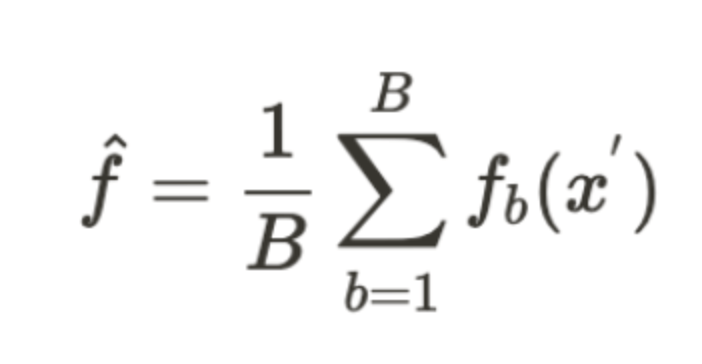
During the training phase of a Random Forest, for each iteration b in 1, 2, … B (where B is the total number of decision trees), the algorithm begins by applying bagging to generate random subsets of the data. Given a training dataset X and Y, it samples n training examples with replacement to form X_b and Y_b. From the available features, N features are randomly selected, and the best split node n is calculated from this subset. Using the chosen split point, the node is divided accordingly. This process of selecting features, identifying the best split, and splitting nodes is repeated until l nodes are generated, and the entire procedure continues until B trees are built. In the testing phase, predictions for unseen samples x’ are made by aggregating (averaging) the outputs from all the individual regression trees.
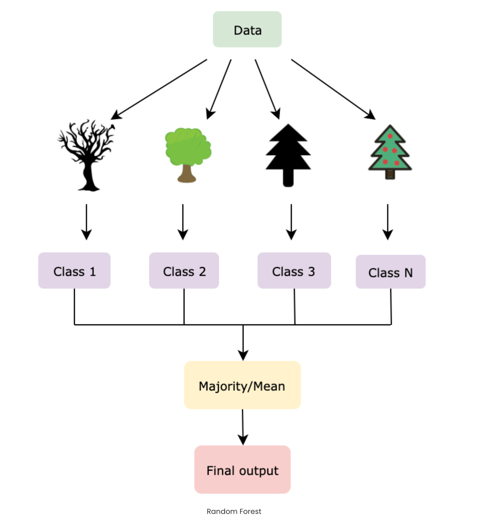
In the case of classification, collect the votes from every tree, and consider the most voted class as the final prediction.
An optimal number of trees in a Random Forest (B) can be chosen based on the size of the dataset, cross-validation, or out-of-bag error. Let’s understand these terms.
Cross-validation is generally used to reduce overfitting in machine learning algorithms. It takes training data and tests it with various test data sets across multiple iterations, denoted by k, hence the name k-fold cross-validation. This can tell us the number of trees based on the k value. Out-of-bag error is the mean prediction error on each training sample x_i, using only those trees that do not have x_i in their bootstrap sample. It’s similar to a leave-one-out cross-validation method.
Computing the feature importance (Feature Engineering)
From here on, let’s understand how Random Forest is coded using the scikit-learn library in Python. Firstly, measuring the feature importance gives a better overview of what features actually affect the predictions. Scikit-learn provides a good feature indicator denoting the relative importance of all the features. This is calculated using the Gini Index or Mean decrease in impurity (MDI) that measures how much the tree nodes that use that feature decrease impurity across all the trees in a forest.
It depicts the contribution made by every feature in the training phase and scales all the scores so that they sum up to 1. This, in turn, helps in shortlisting the important features and dropping the ones that don’t make a huge impact (no impact or less impact) on the model-building process. The reason behind considering only a few features is to reduce overfitting, which usually materializes when there are a good deal of attributes.
Random Forest for Regression: Predicting Continuous Values
While Random Forest is commonly used for classification, it also works exceptionally well for regression problems, where the goal is to predict a continuous numerical value (e.g., predicting house prices, temperatures, or sales).
How It Works
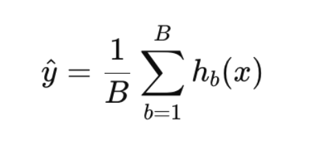
Instead of voting for a class label like in classification, each decision tree in the forest predicts a numeric value. The final output is calculated by averaging the predictions from all individual trees. This averaging reduces variance and leads to more accurate and stable predictions.
Step-by-Step Logic
- Multiple decision trees are trained on random subsets of the dataset (both rows and columns).
- Each tree gives a numeric prediction for the input data point.
- The model averages all predictions from the trees to generate the final output.
If there are B trees in the Random Forest and each tree gives a prediction hb(x), then the final prediction ŷ for an input x is:
Where:
- hb(x) = prediction from the b-th tree
- B = total number of trees in the forest
- ŷ = final predicted value (average of all trees)
RF easily handles nonlinear relationships and also reduces overfitting through averaging. Further, RF models for regression problems are robust to outliers and missing data.
Random Forest Hyperparameters in Scikit-learn
Scikit-learn’s RandomForestClassifier comes with several tunable hyperparameters that allow you to control the model’s complexity, performance, and accuracy. Here’s a breakdown of the most important ones:
1. n_estimators – Number of Trees in the Forest
The number of trees in a Random Forest determines how many individual decision trees will be constructed and aggregated to make predictions. Generally, using a larger number of trees enhances the model’s accuracy and stability, as it allows the algorithm to average more predictions and thereby reduce variance. However, increasing the number of trees also leads to greater computational time and memory consumption. In scikit-learn, the default number of trees was set to 10 in version 0.20, but from version 0.22 onward, it was increased to 100, which strikes a practical balance between performance and training efficiency.
2. criterion – Split Quality Function
This parameter defines the criterion used to evaluate the quality of a potential split at each node in a decision tree. The two most commonly used options are 'gini' and 'entropy'. The 'gini' index measures impurity based on the probability of a randomly chosen element being incorrectly labeled if it were randomly assigned a label according to the distribution in a node. On the other hand, 'entropy' is based on information gain and quantifies the reduction in uncertainty after the split. While 'gini' is the default option and is generally faster to compute, 'entropy' can sometimes lead to slightly better performance depending on the dataset.
3. max_depth – Maximum Tree Depth
The max_depth parameter specifies the maximum depth that each tree in the Random Forest is allowed to grow. If this value is set to None, the tree will keep splitting until all leaf nodes are pure, meaning no further improvement in classification can be made. While deeper trees are capable of capturing more complex patterns in the data, they also run the risk of overfitting. By setting a specific maximum depth, one can help prevent overfitting and reduce the overall computation time, leading to a more efficient and generalizable model.
4. max_features – Features Considered at Each Split
The max_features parameter controls how many features the Random Forest model considers when searching for the best split at each node. For classification tasks, the default setting is either 'auto' or 'sqrt', which selects the square root of the total number of features. Another common option is 'log2', which uses the base-2 logarithm of the number of features. Alternatively, an integer can be specified to indicate the exact number of features to consider, or a float value (e.g., 0.5) can be used to represent a fraction of the total features. Adjusting this parameter helps balance model performance and computational efficiency.
Randomizing the features at each split increases diversity among the trees, helping to reduce correlation and overfitting.
5. min_samples_leaf – Minimum Samples in a Leaf Node
The min_samples_leaf parameter defines the minimum number of samples that a leaf node (the final node in a decision tree) must contain. When this value is set higher, the resulting trees tend to be more conservative, reducing the likelihood of overfitting by avoiding splits that produce very small leaf nodes. This can lead to better generalization, particularly in datasets that are noisy or imbalanced. By default, the value is set to 1, which allows the tree to split as much as possible, offering maximum flexibility but also increasing the risk of overfitting.
6. n_jobs – Number of Parallel Jobs
The n_jobs parameter determines how many CPU cores can be used to train the Random Forest in parallel. By default, setting it to None or 1 runs the training process on a single core. However, setting n_jobs=-1 enables the model to utilize all available CPU cores, which can significantly speed up both training and prediction times. This is especially useful when working with large datasets or models that involve a high number of decision trees.
7. oob_score – Out-of-Bag Evaluation
The oob_score parameter is a Boolean flag that determines whether out-of-bag (OOB) samples should be used to evaluate the model’s performance. OOB samples refer to the data points that are not included in a particular bootstrap sample used to train an individual tree. When oob_score is set to True, the model leverages these excluded samples as a built-in validation set to estimate the generalization error. This approach can save time by eliminating the need for separate cross-validation, making it particularly useful for large datasets. By default, this parameter is set to False.
Coding the algorithm
Step 1: Exploring the data Firstly, from the datasets library in the sklearn package, import the MNIST data.
from sklearn import datasets
mnist = datasets.load_digits()
X = mnist.data
Y = mnist.target
Then, explore the data by printing the data (input) and target (output) of the dataset.
[[ 0.  0.  5. 13.  9.  1.  0.  0.  0.  0. 13. 15. 10. 15.  5.  0.  0.  3.
  15.  2.  0. 11.  8.  0.  0.  4. 12.  0.  0.  8.  8.  0.  0.  5.  8.  0.
   0.  9.  8.  0.  0.  4. 11.  0.  1. 12.  7.  0.  0.  2. 14.  5. 10. 12.
   0.  0.  0.  0.  6. 13. 10.  0.  0.  0.]]
[0]
The input has 64 values, indicating that there are 64 attributes in the data, and the output class label is 0. To prove the same, observe the shapes of X and y, wherein the data and target are stored.
print(mnist.data.shape)
print(mnist.target.shape)

Output:

(1797, 64)
(1797,)
There are 1797 data rows and 64 attributes in the dataset.
Step 2: Preprocessing the data This step includes creating a DataFrame using Pandas. Both the target and data and stored in y and X variables, respectively. pd.Series is used to fetch a 1D array of int datatype. These are a limited set of values that fall under the category data. pd.DataFrame converts the data into a tabular set of values. head() returns the top five values of the DataFrame. Let’s print them.
import pandas as pd

y = pd.Series(mnist.target).astype('int').astype('category')
X = pd.DataFrame(mnist.data)

print(X.head())
print(y.head())
Output:

   0    1    2     3     4     5    6    7    8    9  ...    54   55   56  \
0  0.0  0.0  5.0  13.0   9.0   1.0  0.0  0.0  0.0  0.0 ...   0.0  0.0  0.0
1  0.0  0.0  0.0  12.0  13.0   5.0  0.0  0.0  0.0  0.0 ...   0.0  0.0  0.0
2  0.0  0.0  0.0   4.0  15.0  12.0  0.0  0.0  0.0  0.0 ...   5.0  0.0  0.0
3  0.0  0.0  7.0  15.0  13.0   1.0  0.0  0.0  0.0  8.0 ...   9.0  0.0  0.0
4  0.0  0.0  0.0   1.0  11.0   0.0  0.0  0.0  0.0  0.0 ...   0.0  0.0  0.0

    57   58    59    60    61   62   63
0  0.0  6.0  13.0  10.0   0.0  0.0  0.0
1  0.0  0.0  11.0  16.0  10.0  0.0  0.0
2  0.0  0.0   3.0  11.0  16.0  9.0  0.0
3  0.0  7.0  13.0  13.0   9.0  0.0  0.0
4  0.0  0.0   2.0  16.0   4.0  0.0  0.0

[5 rows x 64 columns]
0    0
1    1
2    2
3    3
4    4
dtype: category
Categories (10, int64): [0, 1, 2, 3, ..., 6, 7, 8, 9]
Segregate the input (X) and the output (y) into train and test data using train_test_split imported from the model_selection package present under sklearn. test_size indicates that 70% of the data points come under training data and 30% come under testing data.
from sklearn.model_selection import train_test_split

X_train, X_test, y_train, y_test = train_test_split(X, y, test_size=0.3)
- X_train is the input in the training data.
- X_test is the input in the testing data.
- y_train is the output in the training data.y_test is the output in the testing data.
Step 3: Creating the Classifier Train the model on the training data using the RandomForestClassifier fetched from the ensemble package present in sklearn. n_estimators parameter indicates that 100 trees are to be included in the Random Forest. The fit() method is to fit the data by training the model on X_train and y_train.
from sklearn.ensemble import RandomForestClassifier

clf=RandomForestClassifier(n_estimators=100)
clf.fit(X_train,y_train)
Predict the outputs using predict() method applied on the X_test data. This gives the predicted values that would be stored in y_pred.
y_pred=clf.predict(X_test)
Check for accuracy using the accuracy_score method imported from the metrics package present in sklearn. The accuracy is estimated against both the actual values (y_test) and the predicted values (y_pred).
from sklearn.metrics import accuracy_score

print("Accuracy: ", accuracy_score(y_test, y_pred))
Output:

Accuracy:  0.9796296296296
This gives 97.96% as the estimated accuracy of the trained Random Forest classifier. A good score indeed!
Step 4: Estimating the feature importance In the previous sections, feature importance has been mentioned as an important characteristic of the Random Forest Classifier. Let’s compute that now.
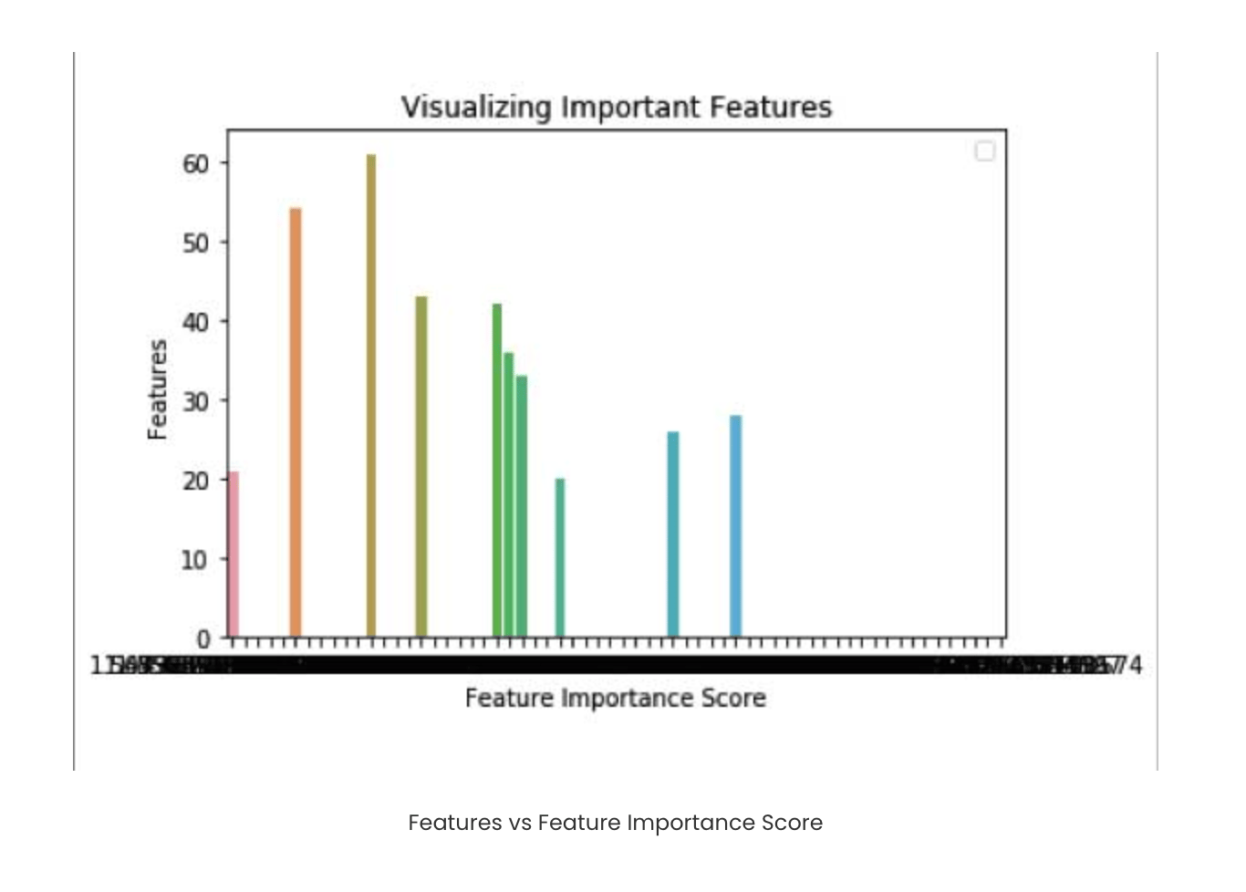
feature_importances_ is provided by the sklearn library as part of the RandomForestClassifier. Extract and sort the values in descending order to print the most significant ones first.
feature_imp=pd.Series(clf.feature_importances_).sort_values(ascending=False)
print(feature_imp[:10])
Output:

21    0.049284
43    0.044338
26    0.042334
36    0.038272
33    0.034299
dtype: float64
The left column denotes the attribute label, i.e., 26th attribute, 43rd attribute, and so on, and the right column is the number indicating the feature importance.
Step 5: Visualizing the feature importance Import the libraries matplotlib, pyplot, and seaborn to visualize the above feature importance outputs. Give the input and output values wherein x is given by the feature importance values, and y is the 10 most significant features out of the 64 attributes, respectively.
import matplotlib.pyplot as plt
import seaborn as sns

%matplotlib inline
sns.barplot(x=feature_imp, y=feature_imp[:10].index)
plt.xlabel('Feature Importance Score')
plt.ylabel('Features')
plt.title("Visualizing Important Features")
plt.legend()
plt.show()
Advantages of Random Forest
- Random Forest is a robust and flexible algorithm suitable for a wide range of problems.
- It can handle missing values effectively without requiring imputation.
- Random Forest can even be adapted for unsupervised learning tasks like clustering using proximity measures.
- The algorithm is relatively easy to understand and implement, especially using libraries like scikit-learn.
- Even with default settings, Random Forest often provides strong baseline performance.
- It helps reduce overfitting by combining predictions from multiple uncorrelated trees.
- Random Forest can be used for feature selection, identifying the most important variables in the data.
- It performs well on high-dimensional datasets, where there are many input features.
Disadvantages of Random Forest
- Training and prediction with Random Forest can be computationally intensive, especially with large datasets.
- The model is hard to interpret, as the logic is spread across many decision trees.
- Using a large number of trees may result in long training times.
- Making predictions can be slower, particularly when real-time responses are needed.
Summary and Conclusion
Random Forest is a powerful, beginner-friendly machine learning algorithm that balances simplicity and performance. By combining the strengths of multiple decision trees, it avoids overfitting and delivers strong results for both classification and regression tasks. Whether you’re working with structured data or solving real-world business problems, Random Forest is a go-to tool in the ML toolkit. If you’re ready to put theory into practice, you can easily spin up a cloud-based environment using DigitalOcean GPU Droplets or deploy your models quickly and scale as needed. It’s the perfect setup for experimenting, training, and testing models like Random Forest—without worrying about hardware limits.
Thanks for learning with the DigitalOcean Community. Check out our offerings for compute, storage, networking, and managed databases.
About the author
With a strong background in data science and over six years of experience, I am passionate about creating in-depth content on technologies. Currently focused on AI, machine learning, and GPU computing, working on topics ranging from deep learning frameworks to optimizing GPU-based workloads.
Still looking for an answer?
This textbox defaults to using Markdown to format your answer.
You can type !ref in this text area to quickly search our full set of tutorials, documentation & marketplace offerings and insert the link!
 This work is licensed under a Creative Commons Attribution-NonCommercial- ShareAlike 4.0 International License.
Become a contributor for community
Get paid to write technical tutorials and select a tech-focused charity to receive a matching donation.

DigitalOcean Documentation
Full documentation for every DigitalOcean product.

Resources for startups and AI-native businesses
The Wave has everything you need to know about building a business, from raising funding to marketing your product.
The developer cloud
Scale up as you grow — whether you're running one virtual machine or ten thousand.

Start building today
From GPU-powered inference and Kubernetes to managed databases and storage, get everything you need to build, scale, and deploy intelligent applications.
