AI Technical Writer

Introduction
XGBoost, short for Extreme Gradient Boosting, is a popular machine learning algorithm known for its speed and accuracy. Created by Tianqi Chen in 2014, it’s widely used in data science and machine learning projects because it works well with many types of data and often gives better results than other algorithms.
In this article, we’ll break down how XGBoost works, what makes it special, and why it’s so commonly used in real-world applications. We’ll also walk through a simple case study using a dataset similar to the one used in the original research, so you can see XGBoost in action.
This guide is ideal for beginners who want to understand the basics of XGBoost, as well as for data practitioners looking for a practical example.
Overview
Improving the accuracy of machine learning models takes more than just fitting algorithms and making predictions. In both industry projects and competitive settings, techniques like feature engineering and ensembling are often used to boost performance.
XGBoost is a prime example of this—it’s an optimized, distributed gradient boosting library known for its speed, flexibility, and portability. It has also become a go-to tool for many data scientists, especially in machine learning competitions on platforms like Kaggle and HackerRank. In fact, around 60% of top-performing solutions in these challenges have used XGBoost as a key component. Of those, about 27% relied solely on XGBoost for training, while the rest combined it with other models—often neural networks—as part of powerful ensemble methods.
To understand how XGBoost works, it’s helpful to first grasp a few key machine learning concepts—namely, supervised learning, decision trees, ensemble learning, and gradient boosting.
Supervised learning is a type of machine learning where an algorithm is trained on a labeled dataset, meaning each data point has both features and a corresponding label. The goal is to learn patterns from this training data and then use the trained model to make predictions on new, unseen data—commonly referred to as test data.
Decision trees are models that make predictions by splitting data into branches based on feature values using a series of true/false questions—much like an if-then-else flowchart. They are used for both classification (predicting categories) and regression (predicting continuous values). The idea is to ask the fewest possible questions to arrive at an accurate prediction.
Gradient Boosted Decision Trees (GBDT) are a type of ensemble learning method that builds a strong model by combining many weak learners—typically shallow decision trees. Ensemble learning, in general, improves performance by combining multiple models. “Gradient Boosting” refers to the process of training these models in sequence, where each new model tries to correct the errors of the ones before it.
Key features and advantages of XGBoost
XGBoost is a flexible framework that supports multiple programming languages, including Python, R, Julia, and C++, making it easy to integrate into a wide range of workflows. It’s also highly portable, working seamlessly across platforms like Digitalocean GPU Droplets, Azure, and Google Colab.
What truly sets XGBoost apart isn’t just its compatibility and portability, but what we can call the “2Ps” — Performance and Processing speed. These two core strengths are the main reasons behind its popularity. Built on the principles of Gradient Boosting, XGBoost takes things a step further by offering faster training and better predictive power than many other ensemble methods like Random Forest. In short, XGBoost is an advanced version of Gradient Boosting that delivers top-tier results thanks to its focus on speed and performance.
Now, what makes this algorithm so fast?
The answer lies behind the concept of parallelization, where the decision trees that create the ensemble are computed using parallel processes. If the algorithm runs on a single processor, then all the cores of the CPU are taken into account. And if it runs in a distributed mode, it ensures to use the maximum available computation power of the system.
Another key reason behind XGBoost’s speed is its smart use of cache optimization. Just like how web browsers store frequently visited pages to load them faster, computer systems use caches to speed up data access. A cache acts as a high-speed storage layer between the CPU and main memory, helping reduce delays in data retrieval.
XGBoost takes advantage of this by caching intermediate calculations and important statistics during training. This means the algorithm doesn’t have to recompute the same things repeatedly, which leads to much faster processing and quicker predictions.
However, this is just the processing part, as a data scientist, one is also concerned about the performance part. In this algorithm, there is a concept of regularization and auto-pruning, which prevents the model from overfitting. This criterion is not present in gradient boosting or GB. A regularization parameter is passed while calling the model, which makes sure overfitting is handled. Hence, the variance of the model is controlled. Also, auto-pruning is a feature that does not lead the model to grow beyond a certain depth. This automatic process of trimming or removing specific branches or subtrees from the gradient boosting decision tree during its construction prevents overfitting, which occurs when a decision tree becomes overly complex and fits the training data too closely, leading to poor generalization on unseen data.
These exceptional features make the model robust, furthermore, XGBoost takes care of the missing values. In the research paper, the author stated that the algorithm seamlessly accommodates sparse feature formats. XGBoost uses a sparsity-aware algorithm to find optimal splits in decision trees, where at each split, the feature set is selected randomly with replacement. When a missing value is encountered, XGBoost can make an informed decision about whether to go left or right in the tree structure based on the available data. This is particularly useful for categorical features with missing values.
Internally, XGBoost learns the best direction to take when a value is missing. This process occurs during the training phase.
Prerequisites and Notes for XGBoost
Before getting started with XGBoost, it’s important to have a basic understanding of Python (or your preferred programming language) and foundational machine learning concepts like supervised learning, classification, regression, and decision trees. Familiarity with libraries like NumPy, pandas, and scikit-learn will also make it easier to work with datasets and models. Since XGBoost is often used for performance tuning and handling large datasets, some experience with model evaluation techniques (like cross-validation and metrics such as accuracy or RMSE) is helpful. Make sure XGBoost is installed in your environment using tools like pip or conda, and check for compatibility with your current system setup.
# Pip 21.3+ is required
pip install -U xgboost
We may also use the Conda packaging manager to install XGBoost:
conda install -c conda-forge py-xgboost
XGBoost Simplified: A Quick Overview

In this section of the tutorial, we will examine in detail a few of XGBoost’s key features.
Boosting
As we learned, XGBoost is a refined iteration of the Boosting algorithm, serving as its foundational core. Boosting is an ensemble modeling method aimed at constructing a robust classifier by combining several weak classifiers. A series of weak learners is combined to build a model. Initially, a model is constructed using the training data. Subsequently, a second model is created with the objective of rectifying any errors made by the first model. This process is iterated, and models are incorporated until either the entire training dataset is predicted accurately or the maximum allowable number of models is reached.
Gradient Boosting
Gradient Boosting is a machine learning technique that focuses on improving the predictive performance of models by training multiple weak learners, typically decision trees, built sequentially. The key idea behind gradient boosting is to correct the errors made by the previous models in an iterative manner.
XGBoost
In this algorithm, decision trees are created sequentially, and weights play a major role in XGBoost. In this approach, each independent variable is initially assigned weights and input into a decision tree for prediction. Variables predicted incorrectly by the tree receive increased weights and are subsequently used in a second decision tree. These individual classifiers then combine to create a robust and more accurate model through ensemble learning.
This iterative boosting approach adapts and improves the model over time, effectively reducing prediction errors and creating a strong ensemble model. It is widely used for both regression and classification tasks and is known for its high predictive accuracy. Popular implementations of gradient boosting include XGBoost, LightGBM, and CatBoost.
XGBoost Parameters
XGBoost has a wide range of parameters that can be tuned to customize the model’s behavior and performance. Let’s examine some of these before identifying which are most important to adjust during training.
- General Parameters:
- booster: Type of boosting model (gbtree, gblinear), the default option is gbtree
- silent: Verbosity level, the valid values are 0 (silent), 1 (warning), 2 (info), 3 (debug). Verbosity is known to print messages
- nthread: Number of parallel CPU threads to use for processing
- Tree Booster Parameters:
- eta (or learning_rate): The Default value is 0.3. This value is the step size shrinkage to prevent overfitting
- max_depth: Maximum depth of the tree
- min_child_weight: Specifies the minimum total weight of all observations necessary in a child node. This parameter controls overfitting however, a higher value can result in underfitting
- subsample: Fraction of observations used for building the tree. This occurs once in every iteration
- colsample_bytree: Fraction of features or columns used for tree building
- lambda (or reg_lambda): L2 regularization
- alpha (or reg_alpha): L1 regularization
- Learning Task Parameters:
- objective: Here, the default value reg:squarederror, Objective defines the loss function which the model aims to reduce (e.g., reg:squarederror for regression, binary: logistic for binary classification)
- eval_metric: Evaluation metric to monitor during training (e.g., rmse for regression, logloss for binary classification)
- Control Parameters:
- num_round (or n_estimators): Number of boosting rounds (trees)
- early_stopping_rounds: If the validation metric doesn’t improve for a specified number of rounds, training stops
- Cross-Validation Parameters:
- num_folds (or nfolds): Number of cross-validation folds
- stratified: Perform stratified sampling for cross-validation. This is used when there is an imbalance in classes in the target variable
These are just a selection of the many parameters available in XGBoost. The choice of parameters depends on the specific problem and the dataset. Careful tuning of these parameters can significantly impact the model’s performance.
- Additional Parameters:
- scale_pos_weight: The default value is 1. This parameter creates a balance of positive and negative weights.
- seed: Random seed for reproducibility.
- gamma: Minimum loss reduction required to make a further partition on a leaf node.
How to best adjust XGBoost parameters for optimal training
Adjusting the parameters for optimal training involves a combination of understanding the problem statement, the dataset, and hyperparameter tuning.
- The first step before diving into hyperparameter tuning is to understand the dataset and the problem statement. This should include initial data preparation, feature engineering, Exploratory Data Analysis (EDA), and settling with the evaluation metric depending upon the problem (classification or regression.)
- Splitting the data into train, test, and validation which can be used to train the model and test its performance on the other two sets. During this process, one should also keep in mind the data leakage issue.Creating the model using the train set, evaluating the model in the test set, and validating the model using the validation set after finding the best hyperparameter. This ensures an unbiased estimate of its performance.
- Creating a base model first with the important or default parameters. This provides a good starting point for the model and later fine-tune the parameters for better performance of the model.
- Next, perform the hyperparameter tuning using techniques like Grid Search, Random Search, or Bayesian optimization (e.g., using libraries like GridSearchCV or RandomizedSearchCV in scikit-learn, or Optuna.)
Among the many parameters XGBoost has, a few of them are most important and need to be considered when deploying a model for training. Here is a list of parameters for optimal training.
-
A. Learning rate (eta)
-
B. Maximum depth (max_depth)
-
C. Number of trees (n_estimators)
-
D. Minimum child weight (min_child_weight)
-
E. Gamma (min_split_loss)
-
F. Subsampling and column subsampling
-
G. Early stopping
-
H. Cross-validation
-
Implement early stopping
-
Experiment with regularization techniques such as L1 and L2.
-
Feature selection and understanding of each feature play a major role. Identifying the main features plays a crucial role. XGBoost has a built-in feature importance score that can help with this. Or we can use tools like SHAP or LIME. These libraries can help find the important features that are contributing positively to the model. And, helps in explaining the black box model.
-
After achieving a satisfactory level of performance with the model, it’s crucial to deploy it for real-world predictions. However, ongoing monitoring is essential because the data environment can evolve over time. This necessitates periodic retraining of the model to account for changing data distributions and new requirements. Even when the model has initially fine-tuned the hyperparameters and struck a balance, it’s common to revisit and potentially revamp the hyperparameters. This iterative process remains a fundamental aspect of Data Science, reflecting its adaptability to dynamic data landscapes.
Please keep in mind that the optimal set of hyperparameters may vary from one problem to another. It’s essential to strike a balance between bias and variance, which is often called a bias-variance trade-off.
Implementation of Extreme Gradient Boosting
Here, we’ll guide you through a step-by-step demonstration of how to use XGBoost to tackle a real-world problem. While the original research paper utilized four datasets, we’ve employed a comparable dataset in this tutorial to showcase XGBoost in action.
| Dataset | Task |
|---|---|
| Allstate | Insurance claim classification |
| Higgs Boson | Event classification |
| Yahoo LTRC | Learning to Rank |
| Criteo | Click-through rate prediction |
Code Demo and explanation
Let us now walk through how to download the dataset, create the model, and utilize it for predicting outcomes on test data. The code below loads the dataset from the web.
Here, we will use a classification problem predicting the click-through Rate. The purpose of click-through rate (CTR) prediction is to predict how likely a person will click on an advertisement or item.
url="https://raw.githubusercontent.com/ataislucky/Data-Science/main/dataset/ad_ctr.csv"
ad_data = pd.read_csv(url)
Explaining the Features of the dataset in brief
The code displays the columns or the features present in the dataset.
ad_data.columns
Variables present in the data set are:
- Clicked on Ad: 1 if the user clicked on the ad, else 0;
- Age: The age of the user
- Daily Time Spent on Site: The daily time spent by the user on the website
- Daily Internet Usage: The Internet usage of the user
- Area Income: Average income of the user
- City: City
- Ad Topic Line: The title of the ad
- Timestamp: The time when the user visited the website
- Gender: Gender of the user
- Country: Country of the user
Data Preparation and Analysis
The below piece of code snippet displays the shape of the dataset, basic info, data types, and value counts of the target column.
# provides the dtypes of the columns
ad_data.dtypes
# prints the shape of the dataframe
ad_data.shape
# displays the columns present in the data
ad_data.columns
# describes the dataframe
ad_data.describe()
Categorical columns need to be converted into numerical columns before feeding them into the model.
gender_mapping = {'Male': 0, 'Female': 1}
ad_data['Gender'] = ad_data['Gender'].map(gender_mapping)
ad_data['Gender'].value_counts(normalize=True)
# Use Label Encoding to convert 'country' to numerical feature
ad_data['Country'] = ad_data['Country'].astype('category').cat.codes
ad_data['Country'].value_counts()
Dropping a few unnecessary columns before model training
ad_data.drop(['Ad Topic Line','City','Timestamp'],axis=1, inplace=True)
Randomly split the training set into train and test subsets.
X_train,X_test,y_train,y_test=train_test_split(X,y,test_size=0.2,random_state=45)
X_train.shape,X_test.shape,y_train.shape,y_test.shape
Model Training: Build an XGBoost Model and Make Predictions
It is imperative to divide our dataset into two distinct sets: the training set, which is used to train our model, and the testing set, which serves to evaluate how effectively our model fits the dataset.
After splitting the data, the base model is trained using default parameters to demonstrate its effectiveness.
# Step 4: Create and train the first basic XGBoost model
model = XGBClassifier()
model.fit(X_train, y_train)
Once trained, we will use the model to predict the test dataset and evaluate its performance on it.
# Step 5: Make predictions
y_pred = model.predict(X_test)
The code below evaluates the model’s performance.
# Step 6: Evaluate the model's performance
accuracy = accuracy_score(y_test, y_pred)
print(f"Accuracy: {accuracy:.2f}")
print(classification_report(y_test, y_pred))
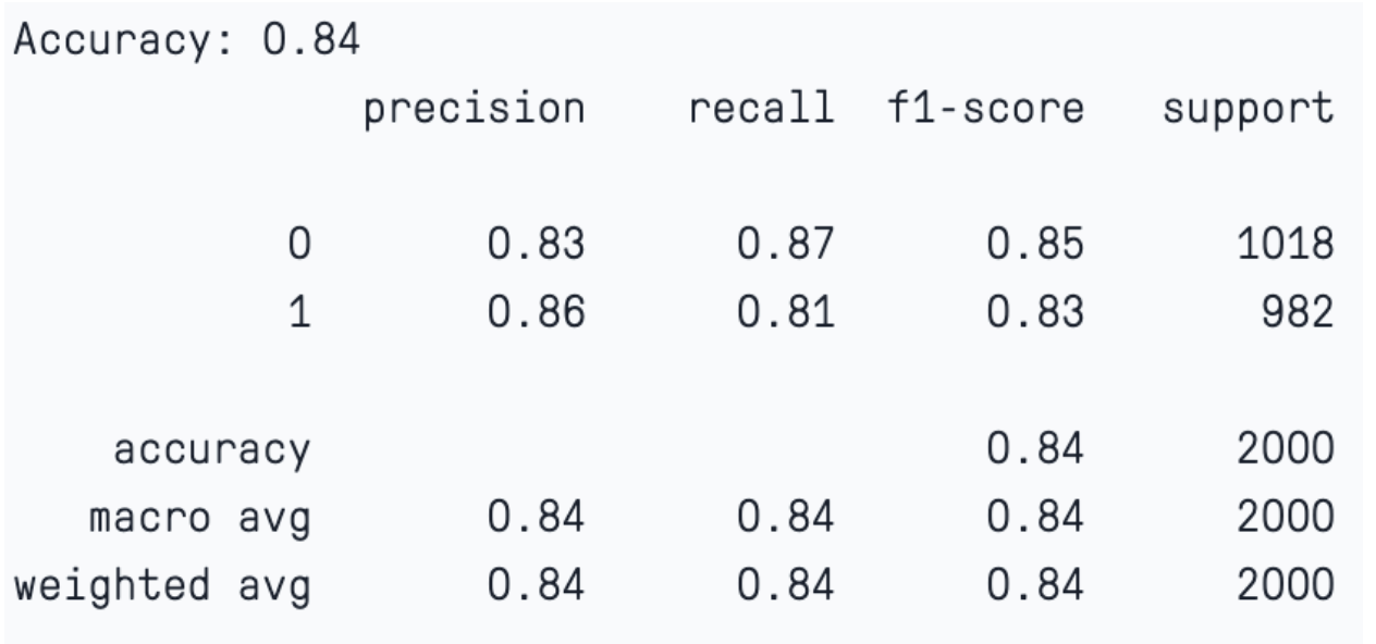
Here, we notice that by providing the default parameters, the model has worked quite well. Please note that accuracy alone may not be a reliable parameter for judging the performance of a machine learning classification model.
Hyperparameter tuning and finding the best parameter
Hyperparameter tuning in XGBoost is a crucial step to optimize the performance of your model. Here are the key steps and considerations for XGBoost hyperparameter tuning:
We will employ GridSearchCV and RandomizedSearchCV to identify the optimal model parameters. The subsequent code demonstrates the training process and parameter tuning.
PARAMETERS = {"subsample":[0.5, 0.75, 1],
"colsample_bytree":[0.5, 0.75, 1],
"max_depth":[2, 6, 12],
"min_child_weight":[1,5,15],
"learning_rate":[0.3, 0.1, 0.03],
"n_estimators":[100]}
model = XGBClassifier(n_estimators=100, n_jobs=-1, eval_metric='error')
"""Initialise Grid Search Model to inherit from the XGBoost Model,
set the of cross validations to 3 per combination and use accuracy
to score the models."""
model_gs = GridSearchCV(model,param_grid=PARAMETERS,cv=3,scoring="accuracy")
model_gs.fit(X_train,y_train)
print(model_gs.best_params_)
Once we get the best parameters from GrisSearchCV, we use them to train and fit the model further.
#Initialise model using best parameters
model = XGBClassifier(objective="binary:logistic",subsample=1,
colsample_bytree=0.5,
min_child_weight=1,
max_depth=12,
learning_rate=0.1,
n_estimators=100)
#Fit the model but stop early if there has been no reduction in error after 10 epochs.
model.fit(X_train, y_train, early_stopping_rounds=5, eval_set=[(X_test, y_test)])
Use the model to predict the target variable on the unseen data.
train_predictions = model.predict(X_train)
model_eval(y_train, train_predictions)
Next, we will again pass the parameters, and this time we will also add the regularization parameter.
params = {'max_depth': [3, 6, 10, 15],
              'learning_rate': [0.01, 0.1, 0.2, 0.3, 0.4],
              'subsample': np.arange(0.5, 1.0, 0.1),
              'colsample_bytree': np.arange(0.5, 1.0, 0.1),
              'colsample_bylevel': np.arange(0.5, 1.0, 0.1),
              'n_estimators': [100, 250, 500, 750],
              'reg_alpha' : [0.1,0.001,.00001],
              'reg_lambda': [0.1,0.001,.00001]

              }
Instantiate the model with 100 estimators.
xgbclf = XGBClassifier(n_estimators=100, n_jobs=-1)
Here, we use RandomizedCV to find the best parameter.
clf = RandomizedSearchCV(estimator=xgbclf,
                             param_distributions=params,
                             scoring='accuracy',
                             n_iter=25,
                             n_jobs=4,
                             verbose=1)
Fit the model, find the best parameter, and use it to predict the target variable.
clf.fit(X_train,y_train)
print("Best hyperparameter combination: ", clf.best_params_)
Repeat the process to train and test the model.
#Initialise model using best parameters from randomized cv
model_new_hyper = XGBClassifier(
                                subsample=0.89,
reg_alpha=0.1,  # L1 regularization (Lasso)
reg_lambda=0.1,  # L2 regularization (Ridge)
colsample_bytree=0.6,
colsample_bylevel=.8,
min_child_weight=1,
max_depth=3,
learning_rate=0.2,
n_estimators=500)
#Fit the model but stop early if there has been no reduction in error after 10 epochs.
model_new_hyper.fit(X_train, y_train, early_stopping_rounds=5, eval_set=[(X_test, y_test)])
In this case, if we check the model evaluation, we notice that the model has maintained a significant bias-variance trade-off. The accuracy of the training and test sets is 87% and 84%, respectively.
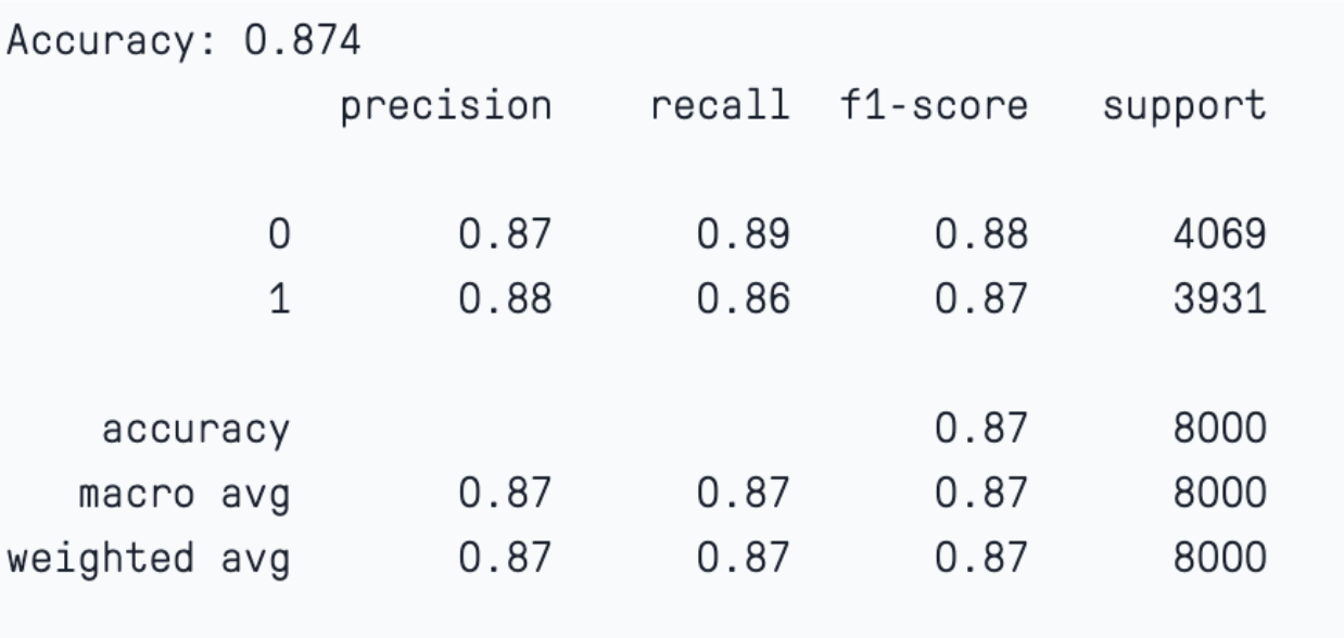
Training set evaluation
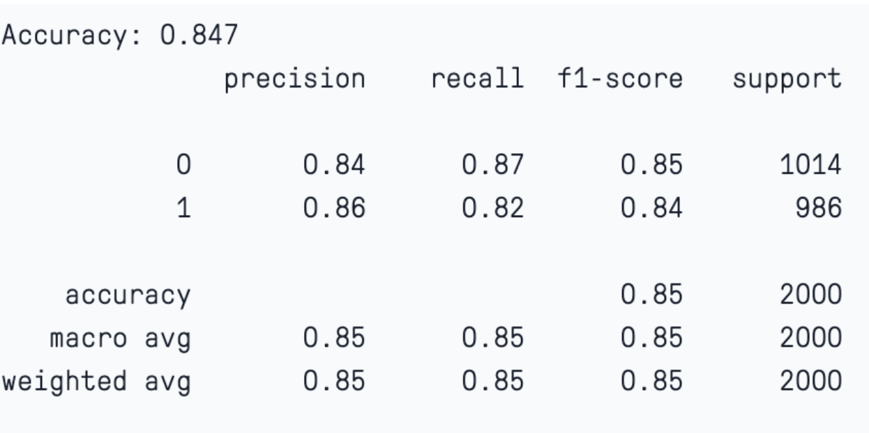
Test set evaluation
XGBoost hyperparameter tuning can be a time-consuming process, but it’s essential for achieving the best model performance. Automated tuning methods can be particularly helpful when dealing with a large number of hyperparameters or when computational resources are limited.
Feature Importance using SHAP
SHAP (SHapley Additive exPlanations) is a game-theoretic approach to understanding each player’s contribution to the final outcome. This, in turn, explains the output of any ML model. ML models, especially ensembles, are considered black box models as they are difficult to interpret. It is harder to determine which are the important predictors for the model.
One of the most used techniques for understanding the feature contribution to the model is utilizing the SHAP values. These values gauge the extent to which individual features, like income, daily internet usage, and Country, influence the model’s predictions. SHAP values provide valuable insights into the significance of specific features and their impact on the final prediction.
In this code demo, we have included SHAP values and their role in the model interpretation.
The code below will install and import the SHAP package from PyPI.
!pip install shap
import shap
We will calculate and visualize the SHAP values and plot the feature importance, feature dependence, and decision plot.
SHAP Explainer
The code below creates an explainer object by providing an XGBoost classification model and then calculates the SHAP value using a testing set.
explainer = shap.Explainer(model)
shap_values = explainer.shap_values(X_test)
shap.summary_plot(shap_values, X_test)
Display the summary_plot.
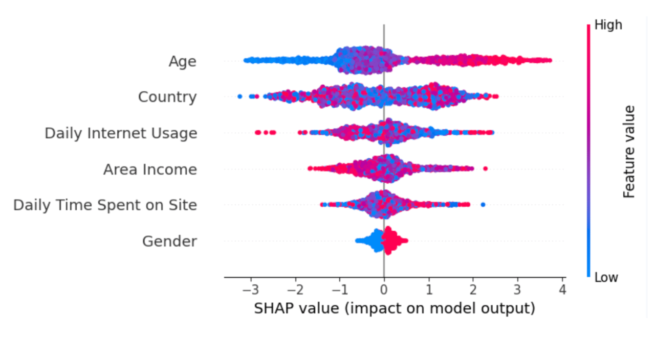
The summary plot shows the feature importance of each feature in the model. The results show that “Age,” “Country,” and “Daily Internet Usage” play major roles as predictors.
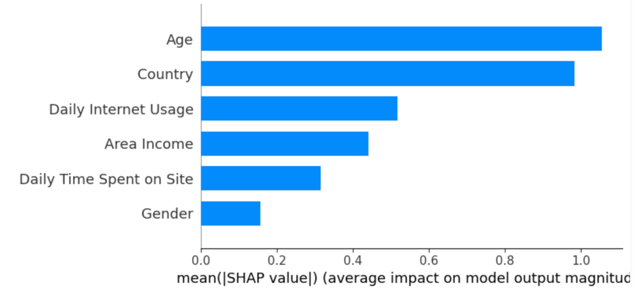
In the below plot,
- The Y-axis represents the feature names arranged in descending order of importance, with the most important features at the top and the least important ones at the bottom.
- The X-axis denotes the SHAP value, which serves as a measure of the extent of change in log odds.
If we examine the “Age” feature and observe a notably positive value, it indicates that Age exerts a substantial positive influence on the output. In other words, when a person’s age is higher, there is a heightened probability that the individual will be more inclined to click on the advertisement. Next, if we look at the feature “Daily Internet usage," we notice that it is mostly high with a negative SHAP value. It means high internet usage tends to negatively affect the output.
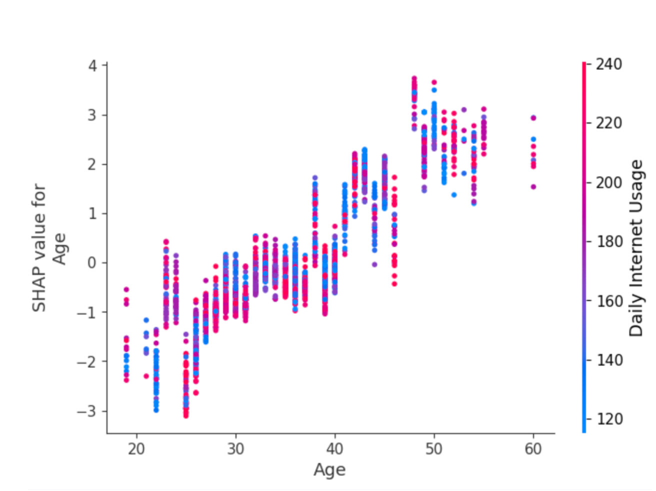
Let us now visualize the “dependence_plot” between the feature “Age” and “Daily Internet usage.” This suggests an interaction effect between Age and Internet Usage.
- Each dot is a single prediction from the dataset, the x-axis is the value of age,
- The y-axis is the SHAP value for that feature, which represents how much knowing that feature’s value changes the model’s output for that sample’s prediction. For this model, the units are log-odds of clicking the ad.
- For example, a 60-year-old with high internet usage is more likely to click on the ad.
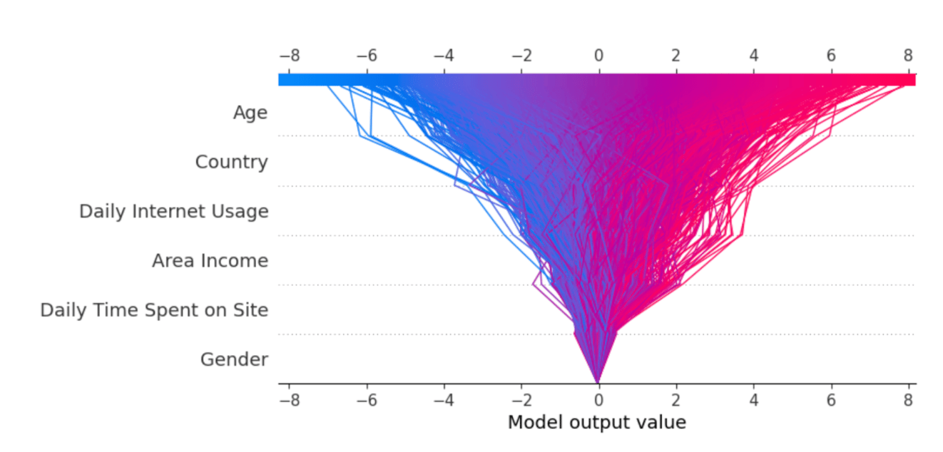
The code below generates a decision plot. The decision plot is displayed in the subsequent output.
expected_value = explainer.expected_value
shap.decision_plot(expected_value, shap_values, X_test)
Every line depicted on the decision plot illustrates the level of influence of individual features on a specific model prediction, thereby elucidating which feature values had the most impact on that prediction.
Saving and Loading XGBoost Models
Saving and loading a trained model using the code snippets below.
model_new_hyper.save_model('model_new_hyper.model')
print("XGBoost model saved successfully.")
# Load the saved XGBoost model
import xgboost as xgb
loaded_model = xgb.Booster()
loaded_model.load_model('model_new_hyper.model')
Now ‘loaded_model’ contains the trained XGBoost model, and can be used for predictions.
Disadvantages of XGBoost
XGBoost is a powerful and popular gradient boosting algorithm. It works by combining multiple decision trees to make a robust model. However, this algorithm does have some disadvantages and limitations.
Complexity: An ensemble model can be computationally demanding by nature, and effectively turning their hyperparameters necessitates extensive experimentation. Training an XGBoost model, especially when dealing with extensive datasets and numerous deep trees, can strain computational resources, which might be a constraint on less capable hardware. In this article, we’ve already covered how this computational complexity can be mitigated through the use of GPUs.
Overfitting: XGBoost is sensitive to noisy data and outliers. While it has built-in regularization to handle overfitting, extreme cases of noise or outliers can still impact its performance. Also, it is a tree-based model, which can sometimes lead to overfitting.
Lack of Interpretability: XGBoost is often called a “black box” model due to its lack of interpretability. We have shown how SHAP values and plots can be used to understand feature importance and impact on the model. However, when a large number of features are used to build the model, understanding the exact decision-making process can be complex.
Despite these disadvantages, XGBoost remains a robust and versatile algorithm in various Kaggle competitions, machine learning, and data science tasks. Understanding these limitations and taking appropriate steps to mitigate them can help maximize the benefits of using XGBoost.
Conclusion
In this blog post, we have presented both the theoretical principles and practical aspects of the Gradient Boosting Algorithm. We have also provided a detailed overview of XGBoost, a scalable tree boosting system widely used by data scientists and providing state-of-the-art results on many problems.
This tutorial outline provides a structured approach to learning and mastering XGBoost, covering everything from installation and data preparation to model training, evaluation, and deployment. We discussed a few disadvantages of the model and how to combat overfitting and underfitting. Also, we included SHAP plots to understand the important features of the model and interpret the model.
Thanks for learning with the DigitalOcean Community. Check out our offerings for compute, storage, networking, and managed databases.
About the author
With a strong background in data science and over six years of experience, I am passionate about creating in-depth content on technologies. Currently focused on AI, machine learning, and GPU computing, working on topics ranging from deep learning frameworks to optimizing GPU-based workloads.
Still looking for an answer?
This textbox defaults to using Markdown to format your answer.
You can type !ref in this text area to quickly search our full set of tutorials, documentation & marketplace offerings and insert the link!
 This work is licensed under a Creative Commons Attribution-NonCommercial- ShareAlike 4.0 International License.
Become a contributor for community
Get paid to write technical tutorials and select a tech-focused charity to receive a matching donation.

DigitalOcean Documentation
Full documentation for every DigitalOcean product.

Resources for startups and AI-native businesses
The Wave has everything you need to know about building a business, from raising funding to marketing your product.
The developer cloud
Scale up as you grow — whether you're running one virtual machine or ten thousand.

Start building today
From GPU-powered inference and Kubernetes to managed databases and storage, get everything you need to build, scale, and deploy intelligent applications.
