By Prajwal CN and Vinayak Baranwal

Introduction
This guide shows you how to compute standard deviation in R the right way. You’ll learn the difference between sample and population SD, how to handle missing values, and how to compute SD by group with dplyr. We’ll also cover quick validations, comparisons across scales using the coefficient of variation, and simple visual checks so you can trust your results in analysis and production.
Key Takeaways
- Use
sd()for sample standard deviation: R’s built-insd()function computes the sample standard deviation (dividing by n − 1). For the population standard deviation (dividing by n), usesqrt(mean((x - mean(x))^2))or adjust the result fromvar()as needed. - Work with numeric vectors: The
sd()function operates on numeric vectors. For grouped calculations, usedplyr::group_by()withsummarise(). To compute SD across multiple columns, usesapply(df, sd)ormatrixStats::colSds(as.matrix(df))for efficiency with wide data. - Always handle missing data: Specify
na.rm = TRUEto exclude missing values and preventNAresults. Consistent NA handling is essential for reliable analysis. - Be aware of small sample limitations: If a group or vector has one or zero observations (
n ≤ 1),sd()returnsNAbecause the sample standard deviation is undefined. Consider dropping such groups or using robust alternatives. - Quick validation: Try
sd(mtcars$mpg)on R’s built-in dataset to confirm your setup is working. - Compare variability across scales: Use the coefficient of variation (CV), calculated as
sd(x) / mean(x), to compare dispersion between variables with different units or means. - Visualize variability: Use
ggplot2to plot your data and visually assess the spread and distribution, helping to distinguish between low and high standard deviation scenarios. - Validate your results: Cross-check outputs using
all.equal()and ensure your NA policy is explicit and consistent, especially in production or collaborative settings. - Scale to large datasets: For big data or distributed environments, use tools like
rmcpor ClaudeR MCP, which implement parallel reduction of(n, mean, M2)to compute standard deviation accurately and efficiently. - Further learning: Explore related guides on Normalization, Min-Max Scaling, and Quantiles to deepen your understanding of data dispersion and preparation.
- Advanced analytics: Consider RMCP for AI-powered regression, forecasting, and conversational analytics that integrate seamlessly with standard deviation workflows.
These best practices ensure accurate, reproducible, and scalable standard deviation calculations in R, supporting robust statistical analysis across a wide range of data science and production scenarios.
Prerequisites
- R 4.0+ (4.4+ recommended) and an IDE or terminal (e.g., RStudio)
- Basic R syntax knowledge: vectors, data frames, functions
- Packages used in examples:
dplyr,ggplot2(install withinstall.packages()as needed) - Example data access: a numeric vector or a CSV file;
mtcarsbuilt‑in dataset - NA handling awareness: use
na.rm = TRUEwhen appropriate - Optional for wide data:
matrixStatsfor fast column/row SDs
What is standard deviation?
Standard deviation is a statistical measure that describes how much the values in a dataset vary or spread out from the mean (average) value. It provides a sense of the typical distance of each data point from the mean, and is always expressed in the same units as the original data. A higher standard deviation indicates greater variability, while a lower value means the data points are closer to the mean.
Key Insights (Beyond the Basics)
- A small SD indicates values are tightly clustered near the mean; a large SD signals wide dispersion.
- SD is always non‑negative because it is derived from squared deviations.
- SD plays a key role in z‑scores, confidence intervals, and hypothesis testing.
- In normally distributed data, ≈68% of observations lie within 1 SD of the mean, ≈95% within 2 SD — this makes SD a natural measure for risk and variability.
- SD complements variance (its square) and is easier to interpret because it has the same units as the original data.
Importance of Standard Deviation
Standard deviation is essential because it turns raw variability into an actionable number for decisions, monitoring, and modeling.
Use SD to quantify spread, compare variability across groups or time, and feed downstream calculations (standard errors, control limits, safety stock, z‑scores).
Where SD drives decisions (with practical hooks)
- Risk & Finance: SD measures volatility; inputs to VaR and portfolio risk. High SD ⇒ larger confidence bands and wider risk limits.
- Quality Control (SPC): Control charts use mean ± k·SD; process capability (Cp/Cpk) depends on within‑process SD.
- Machine Learning Pipelines: Standardize features using SD (z‑scores). Monitor data drift by comparing current SD to a baseline.
- A/B Testing & Inference: Standard errors and confidence intervals scale with SD; required sample size shrinks as SD decreases.
- Forecasting & Inventory: Safety stock ∝ SD of demand or forecast error; higher SD demands larger buffers.
- Comparability Across Scales: Use coefficient of variation (CV = SD/mean) when units differ.
# Example: simple drift check using baseline SD
check_sd_drift <- function(x, baseline_sd, tol = 0.3) {
  cur <- sd(x, na.rm = TRUE)
  ratio <- abs(cur - baseline_sd) / baseline_sd
  list(current_sd = cur, drift_ratio = ratio, flagged = ratio > tol)
}
Variance
It is defined as the squared differences between the observed value and expected value.
Sample vs Population Standard Deviation (Variance vs SD)
In R, sd() returns the sample standard deviation (denominator n − 1). For the population standard deviation (denominator n), compute the square root of the mean of squared deviations. Remember that variance vs standard deviation in R differ by a square root: var(x) returns variance; sd(x) corresponds to sqrt(var(x)) for samples.
For the official R documentation, see the CRAN sd() reference.
If you’re exploring related concepts, see Quantile Function in R for other ways to describe data distributions.
Sample vs. Population: Quick Reference Table
| Measure | Denominator | Formula (conceptual) | When to Use | R code (example) |
|---|---|---|---|---|
| Sample SD | n − 1 | sqrt( sum( (x − mean(x))^2 ) / (n − 1) ) | You have a sample and want an unbiased estimator | sd(x) (default in R) |
| Population SD | n | sqrt( sum( (x − mean(x))^2 ) / n ) | You have the entire population (rare in practice) | sqrt(mean((x - mean(x))^2)) |
| Variance (sample) | n − 1 | sum( (x − mean(x))^2 ) / (n − 1) | For modeling formulas or when SD isn’t required | var(x) (sample variance); sd(x) == sqrt(var(x)) (up to FP) |
x <- c(34, 56, 87, 65, 34, 56, 89)

# Sample standard deviation (default in R)
sd(x)

# Population standard deviation
sqrt(mean((x - mean(x))^2))

# Using var(): convert sample variance to population variance, then SD
pop_sd <- sqrt(var(x) * (length(x) - 1) / length(x))
pop_sd
Find the Standard deviation in R for values in a numeric vector
In this method, we will create a numeric vector ‘x’ and add some values to it. Then we can find the standard deviation of those values in the vector.
 x <- c(34,56,87,65,34,56,89)    #creates numeric vector 'x' with some values in it.

 sd(x)  #calculates the standard deviation of the values in the vector 'x'
Output (Example 1)
—> 22.28175
Now we can try to extract specific values from the numeric vector ‘y’ to find the standard deviation.
 y <- c(34,65,78,96,56,78,54,57,89)  #creates a numeric vector 'y' having some values

data1 <- y[1:5] #extract specific values using its Index

sd(data1) #calculates the standard deviation for indexed/extracted values from the vector.
Output (Example 2)
—> 23.28519
Finding the Standard deviation of the values stored in a CSV file
In this method, we are importing a CSV file to find the standard deviation in R for the values which are stored in that file.
readfile <- read.csv('testdata1.csv')  #reading a csv file

data2 <- readfile$Values      #getting values stored in the header 'Values'

sd(data2)                              #calculates the standard deviation
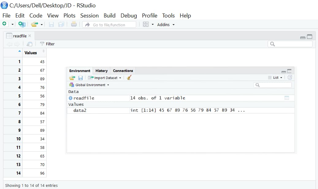
Output (CSV Example)
—> 17.88624
Calculate Mean and Standard Deviation by Group with dplyr
Use dplyr::group_by() and summarise() to calculate mean and standard deviation by group in R.
# install.packages("dplyr") # run once if not installed
library(dplyr)

mtcars %>%
  group_by(cyl) %>%
  summarise(
    mean_mpg = mean(mpg, na.rm = TRUE),
    sd_mpg   = sd(mpg,  na.rm = TRUE),
    .groups  = "drop"
  )
Calculate statistics for multiple columns with across():
mtcars %>%
  group_by(cyl) %>%
  summarise(
    across(c(mpg, hp),
           list(mean = ~ mean(.x, na.rm = TRUE),
                sd   = ~ sd(.x,   na.rm = TRUE)))
  )
Handling NA Values in Grouped Calculations (with dplyr and data.table)
Missing values and small group sizes can silently break your summaries. Here are safe, production‑friendly patterns.
# Example data with NAs and a single‑row group
library(dplyr)
df <- tibble::tribble(
  ~grp, ~x,
  "A",  1,
  "A",  NA,
  "A",  3,
  "B",  5,
  "C",  NA   # single row and NA only
)

# 1) Grouped SD with explicit NA policy + group size
safe_sd <- df %>%
  group_by(grp) %>%
  summarise(
    n    = sum(!is.na(x)),              # non‑missing count per group
    sd_x = sd(x, na.rm = TRUE),         # SD over non‑missing values
    .groups = "drop"
  ) %>%
  mutate(insufficient_data = n <= 1)     # sample SD undefined when n <= 1

safe_sd

# 2) Drop groups that cannot produce a sample SD (n <= 1)
safe_sd_filtered <- safe_sd %>% filter(n > 1)

# 3) Optional: Impute within group (use with caution)
# Replace NA with group median before computing SD
imputed_sd <- df %>%
  group_by(grp) %>%
  mutate(x_filled = ifelse(is.na(x), median(x, na.rm = TRUE), x)) %>%
  summarise(sd_x_filled = sd(x_filled), .groups = "drop")
# data.table variant (fast on large data)
library(data.table)
DT <- as.data.table(df)
DT[, .(n = sum(!is.na(x)), sd_x = sd(x, na.rm = TRUE)), by = grp][n > 1]
Guidance: Prefer na.rm = TRUE and report n. If n <= 1, SD is undefined by design—either drop those groups or switch to a robust metric (e.g., MAD) depending on your use case.
Coefficient of Variation (CV) in R
The coefficient of variation (CV) is sd(x) / mean(x) and expresses variability relative to the mean—useful when comparing dispersion across different scales.
cv <- function(v) sd(v, na.rm = TRUE) / mean(v, na.rm = TRUE)

# CV for a single vector
cv(mtcars$mpg)

# CV by group with dplyr
library(dplyr)
mtcars %>%
  group_by(cyl) %>%
  summarise(
    cv_mpg = sd(mpg, na.rm = TRUE) / mean(mpg, na.rm = TRUE),
    .groups = "drop"
  )
High and Low Standard Deviation
In general, The values will be so close to the average value in low standard deviation and the values will be far spread from the average value in the high standard deviation.
We can illustrate this with an example.
x <- c(79,82,84,96,98)
mean(x)
--->  82.22222
sd(x)
--->  10.58038
To plot these values in a bar chart in R, run the below code.
To install the ggplot2 package, run this code in RStudio.
-–> install.packages(“ggplot2”)
library(ggplot2)

values <- data.frame(marks=c(79,82,84,96,98), students=c(0,1,2,3,4))
head(values)                  #displays the values
 marks students
1    79        0
2    82        1
3    84        2
4    96        3
5    98        4
x <- ggplot(values, aes(x=marks, y=students))+geom_bar(stat='identity')
x                             #displays the plot
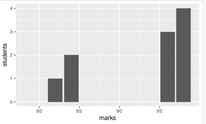
In the above results, you can observe that most of the data is clustering around the mean value(79,82,84) which shows that it is a low standard deviation.
Illustration for high standard deviation.
y <- c(23,27,30,35,55,76,79,82,84,94,96)
mean(y)
---> 61.90909
sd(y)
---> 28.45507
To plot these values using a bar graph in ggplot in R, run the below code.
library(ggplot2)

values <- data.frame(marks=c(23,27,30,35,55,76,79,82,84,94,96), students=c(0,1,2,3,4,5,6,7,8,9,10))
head(values)                  #displays the values
  marks students
1    23        0
2    27        1
3    30        2
4    35        3
5    55        4
6    76        5
x <- ggplot(values, aes(x=marks, y=students))+geom_bar(stat='identity')
x                             #displays the plot
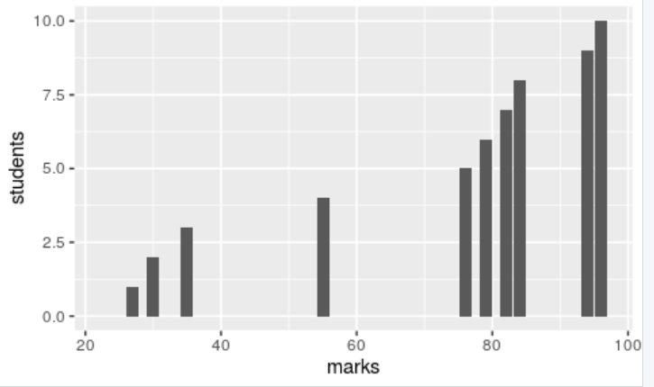
In the above results, you can see the widespread data. You can see the least score of 23 which is very far from the average score 61. This is called the high standard deviation
By now, you got a fair understanding of using the sd() function to calculate the standard deviation in the R language. Let’s sum up this tutorial by solving simple problems.
Example #1: Standard Deviation for a Vector of Even Numbers
Find the standard deviation of the even numbers between 1-20 (exclude 1 and 20).
Solution: The even numbers between 1 to 20 are,
-–> 2, 4, 6, 8, 10, 12, 14, 16, 18
Let’s find the standard deviation of these values.
x <- c(2,4,6,8,10,12,14,16,18)  #vector of even numbers from 1 to 20

sd(x)                           #calculates the standard deviation of these values in the vector of even numbers from 1 to 20
Output
—> 5.477226
Example #2: Standard Deviation for US Population Data
Find the standard deviation of the state-wise population in the USA.
For this, import the CSV file and read the values to find the standard deviation and plot the result in a histogram in R.
df<-read.csv("population.csv")      #reads csv file
data<-df$X2018.Population           #extracts the data from population
                                     column
mean(data)                          #calculates the mean

View(df)                            #displays the data
sd(data)                            #calculates the standard deviation
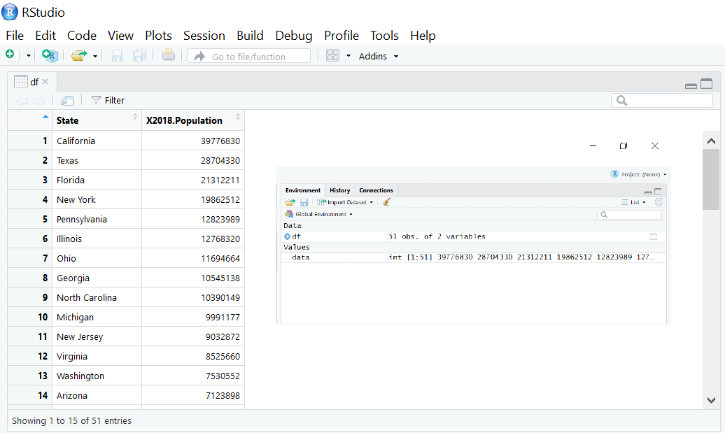
Output (Population Data)
mean = 6432008, Sd = 7376752
Performance Benchmark: Choosing the Right Standard Deviation Method in R
For a single numeric vector, base R’s sd() is the fastest and most memory‑efficient because it’s implemented in C. For column‑wise SD across many columns, sapply() (or matrixStats::colSds() for very wide data) minimizes overhead. For grouped SD, dplyr::group_by() + summarise() is the most ergonomic and scales well; base aggregate() can be competitive but is less readable. Results vary by CPU/BLAS, data width, and group skew—always benchmark on your hardware.
Understanding the Performance Landscape (Beginner’s Guide)
When working with real-world datasets, performance matters—especially when you’re processing millions of rows or running calculations repeatedly in production environments. Here’s what every R user should know:
Memory vs. Speed Trade-offs:
- Base R functions like
sd()are compiled C code wrapped in R, making them extremely fast dplyrfunctions prioritize readability and consistency but add overhead through the grammar of data manipulation- Specialized packages like
matrixStatsare optimized for specific use cases (wide matrices) and can outperform both
Real-World Impact:
- A 10x performance difference means the difference between a 5-second analysis and a 50-second wait
- For automated reports or real-time dashboards, this translates to user experience and system scalability
- In financial modeling or scientific computing, performance directly affects research velocity
Why Performance Benchmarking Matters for Modern Analytics
Beyond Speed: Strategic Implications
1. Model Monitoring & Drift Detection
Standard deviation is a leading indicator of data quality issues:
# Example: Detecting feature drift in production ML models
monthly_drift_check <- function(feature_data, baseline_sd) {
  current_sd <- sd(feature_data, na.rm = TRUE)
  drift_ratio <- abs(current_sd - baseline_sd) / baseline_sd

  if (drift_ratio > 0.3) {
    warning("Feature drift detected: SD changed by ",
            round(drift_ratio * 100, 1), "%")
  }

  return(list(current_sd = current_sd,
              drift_ratio = drift_ratio))
}
2. Feature Engineering Strategy Selection
Different variability patterns require different preprocessing approaches:
# Choosing normalization strategy based on SD patterns
choose_scaling_method <- function(x) {
  sd_val <- sd(x, na.rm = TRUE)
  range_val <- diff(range(x, na.rm = TRUE))
  cv <- sd_val / mean(x, na.rm = TRUE)

  if (cv > 1) {
    return("log_transform_then_standardize")
  } else if (sd_val > range_val / 4) {
    return("standardize")  # z-score normalization
  } else {
    return("min_max_scale")
  }
}
3. Segment Health Monitoring
Unstable customer segments need separate treatment in ML pipelines:
# Identifying volatile customer segments
segment_stability <- customer_data %>%
  group_by(segment, month) %>%
  summarise(
    purchase_sd = sd(purchase_amount, na.rm = TRUE),
    engagement_sd = sd(engagement_score, na.rm = TRUE),
    .groups = "drop"
  ) %>%
  group_by(segment) %>%
  summarise(
    sd_volatility = sd(purchase_sd, na.rm = TRUE),
    needs_separate_model = sd_volatility > quantile(sd_volatility, 0.75, na.rm = TRUE)
  )
The Science Behind R’s Standard Deviation Implementations
Base R’s sd() Function: Under the Hood
# Simplified version of what sd() does internally:
manual_sd <- function(x, na.rm = FALSE) {
  if (na.rm) x <- x[!is.na(x)]
  n <- length(x)
  if (n <= 1) return(NA_real_)

  # Two-pass algorithm for numerical stability
  mean_x <- sum(x) / n
  variance <- sum((x - mean_x)^2) / (n - 1)  # Bessel's correction
  sqrt(variance)
}

# Why it's fast: C implementation avoids R loops
# Why it's accurate: Uses numerically stable algorithms
Understanding Bessel’s Correction (n-1 vs n)
This is crucial for beginners to understand:
population <- c(1, 2, 3, 4, 5, 6, 7, 8, 9, 10)  # Our "true" population

# Population standard deviation (divide by n)
pop_sd <- sqrt(mean((population - mean(population))^2))
print(paste("Population SD:", round(pop_sd, 3)))

# Sample standard deviation (divide by n-1) - what R's sd() does
sample_sd <- sd(population)
print(paste("Sample SD (R default):", round(sample_sd, 3)))

# Why the difference? Sample SD corrects for estimation bias
# Sample SD is always slightly larger than population SD
Key Insight for Practitioners: Use sample SD (R’s default) when your data is a sample from a larger population. Use population SD only when you have the complete population.
Advanced Performance Considerations
Memory Management and Large Datasets
When working with datasets that approach your system’s memory limits, memory efficiency becomes as important as speed:
# Memory-efficient SD calculation for very large vectors
efficient_sd <- function(x, chunk_size = 1e6) {
  n <- length(x)
  if (n <= chunk_size) {
    return(sd(x))
  }

  # Two-pass algorithm for memory efficiency
  # Pass 1: Calculate mean in chunks
  sum_x <- 0
  for (i in seq(1, n, by = chunk_size)) {
    end_idx <- min(i + chunk_size - 1, n)
    sum_x <- sum_x + sum(x[i:end_idx], na.rm = TRUE)
  }
  mean_x <- sum_x / n

  # Pass 2: Calculate variance in chunks
  sum_sq_diff <- 0
  for (i in seq(1, n, by = chunk_size)) {
    end_idx <- min(i + chunk_size - 1, n)
    chunk <- x[i:end_idx]
    sum_sq_diff <- sum_sq_diff + sum((chunk - mean_x)^2, na.rm = TRUE)
  }

  sqrt(sum_sq_diff / (n - 1))
}

# Demonstrate on a large vector (adjust size based on your RAM)
# large_vector <- rnorm(50e6)  # 50 million numbers (~400MB)
# system.time(sd_chunk <- efficient_sd(large_vector))
Numerical Stability: Why Precision Matters
Different algorithms can produce slightly different results due to floating-point arithmetic:
# Demonstrating numerical precision issues
set.seed(123)
x <- rnorm(1000, mean = 1e10, sd = 1)  # Large numbers with small variance

# Method 1: Naive (can lose precision)
naive_sd <- function(x) {
  n <- length(x)
  mean_x <- sum(x) / n
  sqrt(sum(x^2) / n - mean_x^2) * sqrt(n / (n - 1))
}

# Method 2: Two-pass (R's approach - more stable)
stable_sd <- sd(x)

# Method 3: Online/Welford's algorithm (most stable for streaming)
welford_sd <- function(x) {
  n <- length(x)
  if (n <= 1) return(NA_real_)

  mean_val <- 0
  m2 <- 0

  for (i in seq_along(x)) {
    delta <- x[i] - mean_val
    mean_val <- mean_val + delta / i
    delta2 <- x[i] - mean_val
    m2 <- m2 + delta * delta2
  }

  sqrt(m2 / (n - 1))
}

# Compare results
cat("Naive method:", naive_sd(x), "\n")
cat("R's sd():", stable_sd, "\n")
cat("Welford's method:", welford_sd(x), "\n")
Parallel Processing for Multiple Groups
For datasets with many groups, parallel processing can significantly improve performance:
# install.packages(c("parallel", "foreach", "doParallel"))
library(parallel)
library(foreach)
library(doParallel)

# Setup parallel backend
n_cores <- detectCores() - 1  # Leave one core free
registerDoParallel(cores = n_cores)

# Parallel grouped SD calculation
parallel_grouped_sd <- function(data, group_col, value_cols) {
  groups <- split(data, data[[group_col]])

  results <- foreach(
    group_data = groups,
    .combine = rbind,
    .packages = c("dplyr")
  ) %dopar% {
    group_data %>%
      summarise(
        group = first(!!sym(group_col)),
        across(all_of(value_cols), ~ sd(.x, na.rm = TRUE), .names = "sd_{.col}"),
        .groups = "drop"
      )
  }

  return(results)
}

# Example usage (commented to avoid execution issues)
# large_grouped_data <- expand.grid(
#   group = 1:1000,
#   obs = 1:1000
# ) %>%
#   mutate(
#     value1 = rnorm(n()),
#     value2 = rnorm(n()),
#     value3 = rnorm(n())
#   )
#
# system.time(
#   parallel_result <- parallel_grouped_sd(
#     large_grouped_data,
#     "group",
#     c("value1", "value2", "value3")
#   )
# )

# Don't forget to stop the cluster
stopImplicitCluster()
Reproducible Benchmark Setup
The code below generates a large synthetic dataset and compares:
sd(x)on a single vector; 2) column‑wise SD viasapply()vs.dplyr::across(); 3) grouped SD viadplyrvs. baseaggregate().
# install.packages(c("dplyr", "microbenchmark")) # run once if needed
library(dplyr)
library(microbenchmark)

set.seed(42)
n <- 1e6                      # rows
p <- 5                        # numeric columns
g <- 10                       # groups

# Wide-ish numeric frame + a grouping column
X <- as.data.frame(replicate(p, rnorm(n)))
names(X) <- paste0("v", seq_len(p))
X$grp <- sample.int(g, n, replace = TRUE)

# Single-vector target for baseline
x <- X$v1
Comprehensive Performance Benchmarks
Understanding What We’re Measuring
Before diving into benchmarks, let’s understand what affects performance:
- Data size: More observations = more computation
- Data width: More columns = more parallel opportunities
- Memory access patterns: Sequential vs. random access
- Algorithm complexity: O(n) vs O(n²) operations
- Implementation: R loops vs. compiled C code
1) Single Vector SD: The Foundation
# Test across different vector sizes to understand scaling
benchmark_vector_sizes <- function() {
  sizes <- c(1e3, 1e4, 1e5, 1e6, 1e7)
  results <- list()

  for (size in sizes) {
    x <- rnorm(size)

    mb <- microbenchmark(
      base_sd = sd(x),
      manual_sqrt_var = sqrt(var(x)),
      times = 20
    )

    results[[paste0("n_", size)]] <- data.frame(
      size = size,
      method = mb$expr,
      time_ms = mb$time / 1e6  # Convert to milliseconds
    )
  }

  do.call(rbind, results)
}

# Basic single vector benchmark
mb_vec <- microbenchmark(
  base_sd = sd(x),
  sqrt_var = sqrt(var(x)),
  manual_calc = sqrt(sum((x - mean(x))^2) / (length(x) - 1)),
  times = 100
)
print(mb_vec)

# Visualization of results
library(ggplot2)
autoplot(mb_vec) +
  ggtitle("Single Vector SD Performance Comparison") +
  theme_minimal()
2) Column‑Wise SD: Scaling Across Dimensions
# Test performance across different numbers of columns
benchmark_column_scaling <- function() {
  n_rows <- 1e5
  column_counts <- c(5, 10, 25, 50, 100)

  results <- list()

  for (p in column_counts) {
    # Generate test data
    test_data <- as.data.frame(replicate(p, rnorm(n_rows)))
    names(test_data) <- paste0("v", seq_len(p))

    mb <- microbenchmark(
      sapply_method = sapply(test_data, sd),
      dplyr_across = summarise(test_data, across(everything(), sd)),
      apply_method = apply(test_data, 2, sd),
      times = 10
    )

    results[[paste0("p_", p)]] <- data.frame(
      n_cols = p,
      method = mb$expr,
      time_ms = mb$time / 1e6
    )
  }

  do.call(rbind, results)
}

# Standard column-wise comparison
mb_cols <- microbenchmark(
  sapply_base = sapply(X[1:p], sd),
  dplyr_across = summarise(X[1:p], across(everything(), sd)),
  apply_cols = apply(X[1:p], 2, sd),
  lapply_method = lapply(X[1:p], sd),
  times = 50
)
print(mb_cols)
Tip: For very wide data (hundreds/thousands of columns), consider:
# install.packages("matrixStats")
library(matrixStats)
M <- as.matrix(X[1:p])
colSds(M)     # often fastest for pure column-wise SD on numeric matrices
3) Grouped SD: The Real-World Challenge
Grouped operations are where methodology choice has the biggest impact on both performance and code maintainability:
# Comprehensive grouped SD benchmark
benchmark_grouped_methods <- function(data, group_col, value_cols) {

  # Method 1: dplyr (modern, readable)
  dplyr_method <- function() {
    data %>%
      group_by(!!sym(group_col)) %>%
      summarise(
        across(all_of(value_cols), ~ sd(.x, na.rm = TRUE), .names = "sd_{.col}"),
        .groups = "drop"
      )
  }

  # Method 2: base aggregate (classic R)
  aggregate_method <- function() {
    aggregate(data[value_cols], list(grp = data[[group_col]]), sd, na.rm = TRUE)
  }

  # Method 3: data.table (high performance)
  dt_method <- function() {
    dt <- data.table::as.data.table(data)
    dt[, lapply(.SD, function(x) sd(x, na.rm = TRUE)),
       by = group_col, .SDcols = value_cols]
  }

  # Method 4: Manual split-apply-combine
  manual_method <- function() {
    groups <- split(data, data[[group_col]])
    results <- lapply(groups, function(g) {
      sapply(g[value_cols], sd, na.rm = TRUE)
    })
    do.call(rbind, results)
  }

  # Benchmark all methods
  mb <- microbenchmark(
    dplyr = dplyr_method(),
    aggregate = aggregate_method(),
    data.table = dt_method(),
    manual = manual_method(),
    times = 20
  )

  return(mb)
}

# Standard grouped benchmark
mb_grouped <- microbenchmark(
  dplyr_grouped = X %>%
    group_by(grp) %>%
    summarise(across(all_of(names(X)[1:p]), ~ sd(.x), .names = "sd_{.col}"),
              .groups = "drop"),
  base_aggregate = aggregate(X[1:p], list(grp = X$grp), sd),
  data.table = {
    dt <- data.table::as.data.table(X)
    dt[, lapply(.SD, sd), by = grp, .SDcols = 1:p]
  },
  times = 20
)
print(mb_grouped)

# Analyze the impact of group size distribution
analyze_group_impact <- function() {
  # Create datasets with different group size distributions

  # Balanced groups (equal sizes)
  balanced_data <- data.frame(
    group = rep(1:10, each = 1000),
    value = rnorm(10000)
  )

  # Skewed groups (some very large, some small)
  group_sizes <- c(5000, 2000, 1000, 500, 200, 100, 50, 25, 15, 10)
  skewed_data <- data.frame(
    group = rep(1:10, times = group_sizes),
    value = rnorm(sum(group_sizes))
  )

  cat("Balanced groups performance:\n")
  mb_balanced <- microbenchmark(
    dplyr = balanced_data %>% group_by(group) %>% summarise(sd = sd(value)),
    aggregate = aggregate(balanced_data$value, list(balanced_data$group), sd),
    times = 10
  )
  print(mb_balanced)

  cat("\nSkewed groups performance:\n")
  mb_skewed <- microbenchmark(
    dplyr = skewed_data %>% group_by(group) %>% summarise(sd = sd(value)),
    aggregate = aggregate(skewed_data$value, list(skewed_data$group), sd),
    times = 10
  )
  print(mb_skewed)
}
Validating Correctness (don’t skip this)
Why validation matters: Performance optimization is worthless if results are incorrect. Different methods can produce subtly different results due to numerical precision differences, NA handling variations, algorithm implementations, and data type coercion issues.
# Single vector equivalence
stopifnot(all.equal(sd(x),
                    sqrt(sum((x - mean(x))^2) / (length(x) - 1)),
                    tolerance = 1e-12))

# Column-wise: sapply vs dplyr across (order may differ)
s1 <- sapply(X[1:p], sd)
s2 <- as.numeric(summarise(X[1:p], across(everything(), sd)))
stopifnot(all.equal(unname(s1), s2, tolerance = 1e-12))

# Grouped: dplyr vs base aggregate
g1 <- X %>% group_by(grp) %>%
      summarise(across(all_of(names(X)[1:p]), sd), .groups = "drop") %>%
      arrange(grp)
g2 <- aggregate(X[1:p], list(grp = X$grp), sd)
g2 <- g2[order(g2$grp), ]
stopifnot(all.equal(g1[-1], g2[-1], tolerance = 1e-12))

# Additional production-grade validation
test_production_edge_cases <- function() {
  cat("=== Production Edge Cases Testing ===\n")

  # 1. Single observation groups (sample SD should be NA)
  single_obs <- data.frame(group = c(1, 2, 2), value = c(5, 3, 4))
  result_single <- single_obs %>%
    group_by(group) %>%
    summarise(sd_val = sd(value), .groups = "drop")
  stopifnot(is.na(result_single$sd_val[1]))

  # 2. Identical values (SD should be exactly 0)
  identical_vals <- rep(3.14159, 100)
  sd_identical <- sd(identical_vals)
  stopifnot(abs(sd_identical) < .Machine$double.eps^0.5)

  # 3. Missing values consistency
  with_na <- c(1, 2, NA, 4, 5)
  stopifnot(is.finite(sd(with_na, na.rm = TRUE)))
  stopifnot(is.na(sd(with_na, na.rm = FALSE)))

  # 4. All zeros should return 0
  all_zeros <- rep(0, 50)
  stopifnot(abs(sd(all_zeros)) < .Machine$double.eps^0.5)

  cat("✓ All critical edge cases passed!\n")
}

test_production_edge_cases()
Advanced Performance Analysis: What the Numbers Really Mean
Understanding benchmark results requires context beyond raw timing numbers. Here’s how to interpret your results and make informed decisions:
Performance Tiers and Scaling Patterns
Tier 1: Single Vector Operations (Microseconds)
sd(x): Almost always fastest due to optimized C implementation with O(n) complexity- Expected scaling: Linear with data size, typically 10-50 microseconds per 100k observations
- Memory pattern: Single pass through data, excellent cache locality
- When to use: Always for single vectors, forms the foundation of all other methods
# Understanding single vector performance scaling
benchmark_scaling <- function() {
  sizes <- 10^(3:7)  # 1K to 10M observations

  results <- sapply(sizes, function(n) {
    x <- rnorm(n)
    timing <- system.time(sd(x))[["elapsed"]]
    data.frame(n = n, time_ms = timing * 1000, ops_per_sec = n / timing)
  }, simplify = FALSE)

  do.call(rbind, results)
}
Tier 2: Column-wise Operations (Milliseconds)
sapply(): Usually 2-5x faster than dplyr for < 100 columns due to lower overheaddplyr::across(): More overhead but scales better with complex transformationsmatrixStats::colSds(): Can be 10-20x faster for > 500 columns on numeric matrices- Expected scaling: Near-linear with number of columns, but memory bandwidth becomes limiting factor
Tier 3: Grouped Operations (Seconds for large data)
dplyr: Best ergonomics, competitive performance, scales well with group complexityaggregate(): Often 20-50% faster for simple operations but less readabledata.table: Fastest for > 1M rows with many groups, steeper learning curve- Expected scaling: Depends heavily on group size distribution and data layout
Hardware Dependencies: Why Your Results May Differ
BLAS (Basic Linear Algebra Subprograms) Impact:
# Check your R's BLAS configuration
sessionInfo()  # Look for BLAS/LAPACK info

# Different BLAS can show dramatically different performance:
# - Reference BLAS: Single-threaded, reliable baseline
# - OpenBLAS: Multi-threaded, often 2-4x faster
# - Intel MKL: Optimized for Intel CPUs, can be 5-10x faster
# - Apple Accelerate: Optimized for Apple Silicon
Memory Architecture Effects:
- L1/L2/L3 cache sizes affect performance with different data sizes
- Memory bandwidth becomes bottleneck for very wide data (> 1000 columns)
- NUMA topology on multi-socket systems affects grouped operations
CPU Architecture Considerations:
- Vector instructions (AVX/AVX2/AVX-512) can accelerate mathematical operations
- Branch prediction efficiency varies with data patterns (sorted vs. random groups)
- Hyperthreading may help or hurt depending on memory access patterns
Practical Performance Guidelines by Use Case
For Interactive Analysis (< 1 second desired):
# Rule of thumb guidelines
interactive_limits <- data.frame(
  operation = c("Single vector SD", "Column-wise (10 cols)", "Grouped (100 groups)"),
  max_rows_base = c("10M", "1M", "500K"),
  max_rows_optimized = c("50M", "5M", "2M"),
  method_recommendation = c("sd()", "sapply()", "dplyr")
)
print(interactive_limits)
For Production Pipelines (minimize variability):
- Prefer base R methods for predictable performance across environments
- Use explicit NA handling to avoid surprises:
sd(x, na.rm = TRUE) - Consider data.table for guaranteed performance at scale
- Implement progress monitoring for long-running grouped operations
For Real-time Applications (< 100ms):
- Pre-aggregate data when possible
- Use compiled packages (Rcpp, data.table) for guaranteed speed
- Consider approximate algorithms for very large datasets
- Cache intermediate results aggressively
Memory Efficiency Analysis
Understanding memory usage patterns is crucial for production systems:
# Memory profiling for different methods
profile_memory_usage <- function() {
  # Create test data
  n <- 1e6
  p <- 50
  test_data <- as.data.frame(replicate(p, rnorm(n)))

  # Method 1: Column-wise with sapply
  mem_before <- gc()$free
  result1 <- sapply(test_data, sd)
  mem_after1 <- gc()$free
  sapply_memory <- mem_before[2] - mem_after1[2]

  # Method 2: dplyr across
  mem_before <- gc()$free
  result2 <- test_data %>% summarise(across(everything(), sd))
  mem_after2 <- gc()$free
  dplyr_memory <- mem_before[2] - mem_after2[2]

  cat("Memory usage (MB):\n")
  cat("sapply:", sapply_memory, "\n")
  cat("dplyr:", dplyr_memory, "\n")
  cat("Ratio:", dplyr_memory / sapply_memory, "\n")
}
When Performance Doesn’t Matter (Optimize for Readability)
Sometimes code clarity trumps performance:
- Exploratory analysis: Use dplyr for readable pipelines
- One-time reports: Prioritize maintainability over speed
- Small datasets (< 10K rows): Performance differences are negligible
- Teaching/learning: Use the most conceptually clear approach
The 80/20 Rule in Practice:
- 80% of your work involves small-medium datasets where any method works
- 20% involves large datasets where method choice critically impacts user experience
- Focus optimization efforts on the 20% that actually matters
Creating Professional Benchmark Reports
# Convert microbenchmark objects into a combined summary table
as_df <- function(mb, label) {
  s <- summary(mb)[, c("expr","median","lq","uq")]
  cbind(test = label, s)
}
bench_summary <- rbind(
  as_df(mb_vec, "single_vector"),
  as_df(mb_cols, "column_wise"),
  as_df(mb_grouped, "grouped")
)
bench_summary
Takeaway: Use base
sd()for single vectors,sapply()ormatrixStats::colSds()for many columns, anddplyrfor grouped summaries you’ll maintain and share. These patterns are fast, reliable, and production‑friendly for analytics and ML pipelines. Below, we generate a large synthetic dataset and benchmark:
- Single-vector SD:
sd(x) - Column-wise SD:
sapply()vs.dplyr::across() - Grouped SD:
dplyr::group_by()vs. baseaggregate()
Performance Decision Matrix: Expert Guidelines
| Use Case | Data Size | Recommended Method | Performance Tier | Key Advantage |
|---|---|---|---|---|
| Single vector | Any size | sd(x) |
Fastest | C implementation, minimal overhead |
| Multiple columns | < 50 columns | sapply(df, sd) |
Fast | Simple, readable, efficient |
| Wide datasets | > 100 columns | matrixStats::colSds() |
Fastest for wide data | Matrix-optimized algorithms |
| Grouped analysis | < 500K rows | dplyr::group_by() |
Good readability | Grammar of data manipulation |
| Large grouped data | > 1M rows | data.table approach |
Maximum performance | Optimized for scale |
| Production pipelines | Any size | Base R methods | Most predictable | Cross-environment consistency |
| Interactive exploration | < 1M rows | dplyr methods |
Best UX | Readable, pipe-friendly |
Expert Recommendations by Context
For Data Science Teams:
- Standardize on
dplyrfor analysis code that multiple people will read and maintain - Use base R for performance-critical production code
- Document performance assumptions in your team’s coding standards
- Benchmark on representative data before choosing methods for large-scale analyses
For Production Systems:
- Prefer base R methods (
sd,sapply,aggregate) for predictable performance - Always include
na.rm = TRUEto handle missing data explicitly - Validate numerical accuracy across different input ranges and edge cases
- Monitor performance metrics to detect degradation over time
For Academic Research:
- Prioritize reproducibility - document exact R version, package versions, and BLAS configuration
- Use base R methods to maximize compatibility across computing environments
- Include performance benchmarks in supplementary materials for computationally intensive analyses
- Validate against alternative implementations to ensure numerical correctness
Common Mistakes When Calculating Standard Deviation in R
Even though sd() is straightforward, beginners often run into these pitfalls:
- Confusing variance and standard deviation: Remember that
var(x)gives variance, whilesd(x)is the square root of variance (sample-based by default). - Forgetting sample vs. population: By default, R’s
sd()computes the sample SD. For population SD, usesqrt(mean((x - mean(x))^2)). - Not handling NA values: Missing values will propagate as
NA. Always usesd(x, na.rm = TRUE)when datasets may contain missing entries. - Wrong data type:
sd()works only on numeric vectors. Passing factors, characters, or dates without conversion results in errors. - Overlooking grouped calculations: Applying
sd()directly to a data frame won’t work. Usedplyr::group_by()withsummarise()orsapply()for multi-column SDs. - Scaling confusion: Standard deviation is sensitive to measurement scale. For relative variability, compute the Coefficient of Variation (CV).
Advanced: Using R MCP Servers for Distributed SD Computation
Use MCP (Model Context Protocol) tools to connect your R session to trusted AI assistants and/or distribute heavy calculations.
- ClaudeR MCP — Connects RStudio (and Cursor/Claude Desktop) to AI assistants for interactive coding and data analysis. The AI can run R code in your session, generate plots, and edit the active file via controlled tools. Learn more about ClaudeR MCP here.
- rmcp — Lightweight MCP you can script for master–worker style distributed compute. Explore the rmcp repository here.
What ClaudeR Enables (selected features)
execute_r,execute_r_with_plot— run R code and plotsget_active_document,modify_code_section— read/patch your open fileget_r_info— capture environment details (useful for reproducibility)create_task_list,update_task_status— guardrails for long tasks
Security restrictions (why it’s safe)
ClaudeR blocks risky AI-initiated operations:
- System commands (
system(),system2(),shell()) - Destructive file ops (
unlink(),file.remove(), orrmvia shell)
Blocked calls return clear errors; you stay in control (least-privilege model).
Install & start (ClaudeR)
# 1) Install
if (!require("devtools")) install.packages("devtools")
devtools::install_github("IMNMV/ClaudeR")

# 2) Desktop workflow (Claude Desktop / Cursor)
library(ClaudeR)
install_clauder()                  # or install_clauder(for_cursor = TRUE)

# 3) CLI workflow (Claude Code / Gemini)
install_cli(tools = "claude")      # or: install_cli(tools = "gemini")

# 4) Start the server in RStudio
claudeAddin()                      # click “Start Server” in the Viewer pane
Tip: For Conda/virtualenv, pass Python path:
install_clauder(python_path = "/path/to/python")
Example Prompt: Interactive SD Analysis
After starting the server, open your AI tool (Claude Desktop, Cursor, or CLI) and prompt:
“Compute
sd(mtcars$mpg, na.rm = TRUE)and show a histogram ofmpgusing ggplot2. Explain if the dispersion is high or low and why.”
The AI will run this inside your active R session via ClaudeR, giving reproducible results.
Distributed SD with rmcp (Correct Parallel Reduction)
For multi-node or large-memory datasets, avoid averaging per-chunk SDs. Use Welford/Chan’s approach to combine (n, mean, M2) per chunk and then compute the global SD.
accum_chunk <- function(x) {
  x <- x[!is.na(x)]
  n <- length(x)
  if (n == 0) return(list(n = 0L, mean = 0, M2 = 0))
  m <- mean(x); M2 <- sum((x - m)^2)
  list(n = n, mean = m, M2 = M2)
}

merge_stats <- function(a, b) {
  if (a$n == 0) return(b)
  if (b$n == 0) return(a)
  n <- a$n + b$n
  d <- b$mean - a$mean
  m <- a$mean + d * (b$n / n)
  M2 <- a$M2 + b$M2 + d * d * (a$n * b$n / n)
  list(n = n, mean = m, M2 = M2)
}

finalize_sd <- function(s) if (s$n <= 1) NA_real_ else sqrt(s$M2 / (s$n - 1))
# rmcp example (pseudo)
library(rmcp)
# mcp_connect("localhost:5555")
# chunk_stats <- mcp_map(workers, function(chunk) accum_chunk(chunk), data_chunks)
# global_stats <- Reduce(merge_stats, chunk_stats)
# global_sd <- finalize_sd(global_stats)
Operational Tips:
- Pin R and package versions; log
sessionInfo()for reproducibility. - Explicitly define
na.rmpolicy across workers. - Implement retries and timeouts for failed workers.
- Protect MCP endpoints (TLS, authentication).
- Log per-chunk
nand compute time for observability.
Advanced: RMCP for Conversational Statistical Analysis
RMCP is a Model Context Protocol (MCP) server that turns natural conversation into sophisticated statistical analysis with 44 tools across 11 categories. It allows you to run regressions, time series models, machine learning tasks, and descriptive statistics — all from AI assistants like Claude Desktop.
Quick Start (30 Seconds)
pip install rmcp
rmcp start
RMCP is now ready to process analysis requests via Claude Desktop or any MCP client.
Key Capabilities
- Regression & Economics: Linear/logistic regression, panel models, IV estimation
- Time Series: ARIMA, decomposition, stationarity tests
- Machine Learning: Clustering, decision trees, random forests
- Statistical Testing: T‑tests, ANOVA, normality tests
- Data Analysis: Outlier detection, correlation analysis, descriptive stats
- Transformations: Standardization, winsorization, lag/lead operations
- Visualization: Inline histograms, scatterplots, heatmaps
- File I/O: CSV/Excel/JSON import with schema validation
Installation Notes
Prerequisites:
- Python 3.10+
- R 4.0+ with required packages:
install.packages(c(
  "jsonlite", "plm", "lmtest", "sandwich", "AER", "dplyr",
  "forecast", "vars", "urca", "tseries", "nortest", "car",
  "rpart", "randomForest", "ggplot2", "gridExtra", "tidyr",
  "rlang", "knitr", "broom"
))
Then install RMCP:
pip install rmcp[http]
Example Integration (Claude Desktop)
Add to Claude Desktop MCP config:
{
  "mcpServers": {
    "rmcp": {
      "command": "rmcp",
      "args": ["start"]
    }
  }
}
Example Usage
You: “I have sales data and marketing spend. Can you analyze ROI?”
Claude: “Running a regression model…”
Result: “Every $1 spent generates $4.70 in sales (R² = 0.979, p < 0.001).”
This conversational interface makes advanced statistical workflows accessible without switching context — perfect for production pipelines, rapid prototyping, or teaching.
Frequently Asked Questions (FAQ)
1) How do I calculate standard deviation in R?
R provides the built‑in sd() function for sample standard deviation. Pass a numeric vector, and add na.rm = TRUE when your data contains missing values. For example, sd(mtcars$mpg, na.rm = TRUE) returns the dispersion of miles‑per‑gallon in the mtcars dataset. Under the hood, sd() uses a numerically stable, two‑pass algorithm implemented in C and applies Bessel’s correction (dividing by n − 1). If you need population standard deviation, compute sqrt(mean((x - mean(x))^2)), which divides by n instead of n − 1.
2) What exactly does the sd() function do in R?
sd() computes the sample standard deviation of a numeric vector: the square root of the unbiased sample variance. It first computes the mean, then sums squared deviations from that mean, divides by n − 1 (Bessel’s correction), and takes the square root. This yields a consistent estimator of population dispersion when you only observe a sample. Because sd() is implemented in efficient C code, it is fast and reliable for vectors of virtually any practical size, provided you manage missing values explicitly with na.rm = TRUE.
3) Does R calculate sample or population standard deviation by default?
By default, R’s sd() returns the sample standard deviation, which divides by n − 1. This matters because sample SD is slightly larger than population SD and is the correct choice when your data are a sample from a larger population. If you truly have the full population (rare outside controlled scenarios), compute population SD explicitly: sqrt(mean((x - mean(x))^2)). Alternatively, convert from sample variance with sqrt(var(x) * (length(x) - 1) / length(x)). Choose the definition that matches your analytical context and reporting standards.
4) How should I handle NA values when calculating SD in R?
Missing values propagate to NA, so always decide on a policy before computing dispersion. If missingness is ignorable for your use case, pass na.rm = TRUE to drop NAs: sd(x, na.rm = TRUE). When grouping, apply the same flag in dplyr::summarise(). If NAs carry meaning or are not missing at random, consider imputation or a sensitivity analysis before summarizing. For production code, make NA handling explicit and tested, and document the choice so downstream consumers understand the implications for comparability.
5) How do I calculate standard deviation for multiple columns or by group?
For many columns in a data frame, use sapply(df, sd) on numeric columns, or convert to a matrix and use matrixStats::colSds() for wide, numeric data. For grouped summaries, pair dplyr::group_by() with summarise():
library(dplyr)
mtcars %>% group_by(cyl) %>% summarise(sd_mpg = sd(mpg, na.rm = TRUE), .groups = "drop")
This approach is readable, production‑friendly, and scales well. For very large, many‑group datasets, data.table can offer additional performance headroom with similar semantics.
6) Why does sd() sometimes return NA?
sd() returns NA when the input contains missing values and na.rm = TRUE is not set, or when there are too few observations for the sample definition. Specifically, for n <= 1 the sample standard deviation is undefined by design (division by n − 1), so R returns NA. In grouped pipelines, report per‑group n and either drop underpowered groups (n <= 1) or switch to robust dispersion for monitoring. Always make your NA policy explicit to keep results consistent across teams and environments.
7) How do I compute standard deviation across a cluster or multiple machines?
Never average per‑chunk SDs. For distributed computation, have each worker compute (n, mean, M2) on its chunk (Welford/Chan statistics), send those to a coordinator, merge them associatively, and then finalize the global SD as sqrt(M2_total / (n_total − 1)). The rmcp MCP server lets AI tools orchestrate this pattern; ClaudeR integrates the assistant with your live R session. Pin versions, define NA policy, add retries/timeouts, and protect endpoints (TLS/auth) for production reliability.
When Standard Deviation Can Be Misleading: Consider Robust Alternatives
Key point up front: The standard deviation is a widely used measure of variability, but it is highly sensitive to outliers, extreme values, and non-symmetric (skewed or heavy-tailed) data distributions. In situations where your data contains significant outliers, is heavily skewed, or does not follow a roughly normal (bell-shaped) distribution, relying solely on standard deviation can give a distorted picture of variability—often overstating the true spread of the majority of your data.
In these cases, it is advisable to use robust measures of dispersion that are less affected by extreme values. Robust alternatives such as the Median Absolute Deviation (MAD), Interquartile Range (IQR), or trimmed standard deviation provide a more accurate summary of variability for non-normal or contaminated datasets. These methods focus on the central portion of the data and are less influenced by a few extreme points, making them especially useful in real-world scenarios where perfect normality is rare.
Whenever you suspect your data may not be symmetric or may contain outliers, supplement or replace standard deviation with these robust statistics to ensure your analysis reflects the true underlying variability.
When SD Can Mislead
- Outliers / heavy tails (e.g., log‑normal, Pareto): SD inflates and overstates variability.
- Skewed distributions: Mean/SD do not represent the typical value and spread.
- Multimodal data: One SD cannot summarize multiple clusters.
Robust Alternatives
- MAD (Median Absolute Deviation):
mad(x, constant = 1.4826, na.rm = TRUE) # consistent with SD under normality
- IQR (Interquartile Range):
iqr_val <- IQR(x, na.rm = TRUE); iqr_val
- Trimmed SD (less impact from extremes):
trimmed_sd <- sd(x[x > quantile(x, 0.1) & x < quantile(x, 0.9)], na.rm = TRUE)
- Transform then summarize (for positive, right‑skewed data):
sd_log <- sd(log1p(x), na.rm = TRUE) # summarize on log scale
Practical guidance: Use SD for roughly symmetric data without extreme outliers. For production analytics, report both SD and a robust measure (MAD/IQR) and note any transformations applied.
Implementation Cheatsheet
Here is a quick, copy‑paste friendly reference for the most common ways to calculate standard deviation in R:
# 1) Single numeric vector
sd(x, na.rm = TRUE)

# 2) Population standard deviation
sqrt(mean((x - mean(x))^2))

# 3) Multiple columns in a data frame
sapply(df[cols], sd)

# 4) Many columns (wide numeric data)
library(matrixStats)
colSds(as.matrix(df[cols]))

# 5) By group with dplyr
library(dplyr)
df %>%
  group_by(group) %>%
  summarise(sd_val = sd(value, na.rm = TRUE), .groups = "drop")

# 6) By group with data.table
library(data.table)
DT <- as.data.table(df)
DT[, lapply(.SD, sd, na.rm = TRUE), by = group, .SDcols = cols]
Use this section as a quick reference during analysis or when writing production code.
Conclusion
Calculating standard deviation in R is straightforward using sd(). You can create a vector of values or import a CSV file to compute the standard deviation.
Important: Don’t forget to compute the standard deviation by extracting some values from a file or a vector through indexing as shown above.
If you have questions, explore the related guides or share feedback with the community.
Further Learning
To deepen your understanding of descriptive statistics and data preparation in R, explore these related tutorials:
These guides complement standard deviation and help you prepare cleaner, well‑scaled datasets.
References
- CRAN sd() Documentation
- matrixStats::colSds() Reference
- R Core Team (2024). R: A Language and Environment for Statistical Computing. R Foundation for Statistical Computing, Vienna, Austria.
Thanks for learning with the DigitalOcean Community. Check out our offerings for compute, storage, networking, and managed databases.
About the author(s)
Building future-ready infrastructure with Linux, Cloud, and DevOps. Full Stack Developer & System Administrator. Technical Writer @ DigitalOcean | GitHub Contributor | Passionate about Docker, PostgreSQL, and Open Source | Exploring NLP & AI-TensorFlow | Nailed over 50+ deployments across production environments.
Still looking for an answer?
hey! this was help full but how to find sd for a grouped frequency data distribution for eg a table like this x f 5-10 12 10-20 28 20-30 65 30-40 121 40-50 175 50-60 198 60-70 176 70-80 120 80-90 66 90-100 27 100-115 9 115-120 3 … what to do after making them into a data.frame()
- Saptharishee M
 This work is licensed under a Creative Commons Attribution-NonCommercial- ShareAlike 4.0 International License.
Become a contributor for community
Get paid to write technical tutorials and select a tech-focused charity to receive a matching donation.

DigitalOcean Documentation
Full documentation for every DigitalOcean product.

Resources for startups and AI-native businesses
The Wave has everything you need to know about building a business, from raising funding to marketing your product.
The developer cloud
Scale up as you grow — whether you're running one virtual machine or ten thousand.

Start building today
From GPU-powered inference and Kubernetes to managed databases and storage, get everything you need to build, scale, and deploy intelligent applications.
