
Introduction
Neural networks are used as a method of deep learning, one of the many subfields of artificial intelligence. They were first proposed around 70 years ago as an attempt at simulating the way the human brain works, though in a much more simplified form. Individual ‘neurons’ are connected in layers, with weights assigned to determine how the neuron responds when signals are propagated through the network. Previously, neural networks were limited in the number of neurons they were able to simulate, and therefore the complexity of learning they could achieve. But in recent years, due to advancements in hardware development, we have been able to build very deep networks, and train them on enormous datasets to achieve breakthroughs in machine intelligence.
These breakthroughs have allowed machines to match and exceed the capabilities of humans at performing certain tasks. One such task is object recognition. Though machines have historically been unable to match human vision, recent advances in deep learning have made it possible to build neural networks which can recognize objects, faces, text, and even emotions.
In this tutorial, you will implement a small subsection of object recognition—digit recognition. Using TensorFlow, an open-source Python library developed by the Google Brain labs for deep learning research, you will take hand-drawn images of the numbers 0-9 and build and train a neural network to recognize and predict the correct label for the digit displayed.
While you won’t need prior experience in practical deep learning or TensorFlow to follow along with this tutorial, we’ll assume some familiarity with machine learning terms and concepts such as training and testing, features and labels, optimization, and evaluation. You can learn more about these concepts in An Introduction to Machine Learning.
Prerequisites
To complete this tutorial, you’ll need:
- A local Python 3.6 development environment, including pip, a tool for installing Python packages, and venv, for creating virtual environments.
Note: TensorFlow requires a minimum Python version of 3.5 and supports versions up to 3.8. Older or newer versions of Python are not supported. This tutorial is designed to work with TensorFlow versions 1.4.0-1.15.5 with Python 3.6. Newer or older version of either will likely result in installation or runtime errors. For a full list of version requirements for Windows, macOS, and Linux, visit the Install TensorFlow with pip page on the TensorFlow site.
Step 1 — Configuring the Project
Before you can develop the recognition program, you’ll need to install a few dependencies and create a workspace to hold your files.
We’ll use a Python 3 virtual environment to manage our project’s dependencies. Create a new directory for your project and navigate to the new directory:
- mkdir tensorflow-demo
- cd tensorflow-demo
Execute the following commands to set up the virtual environment for this tutorial:
- python3 -m venv tensorflow-demo
- source tensorflow-demo/bin/activate
Next, install the libraries you’ll use in this tutorial. We’ll use specific versions of these libraries by creating a requirements.txt file in the project directory which specifies the requirement and the version we need. Create the requirements.txt file:
- touch requirements.txt
Open the file in your text editor and add the following lines to specify the Image, NumPy, and TensorFlow libraries and their versions:
requirements.txtimage==1.5.20
numpy==1.14.3
tensorflow==1.4.0
Save the file and exit the editor. Then install these libraries with the following command:
- pip install -r requirements.txt
With the dependencies installed, we can start working on our project.
Step 2 — Importing the MNIST Dataset
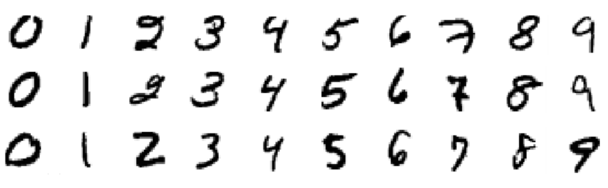
The dataset we will be using in this tutorial is called the MNIST dataset, and it is a classic in the machine learning community. This dataset is made up of images of handwritten digits, 28x28 pixels in size. Here are some examples of the digits included in the dataset:
Let’s create a Python program to work with this dataset. We will use one file for all of our work in this tutorial. Create a new file called main.py:
- touch main.py
Now open this file in your text editor of choice and add this line of code to the file to import the TensorFlow library:
import tensorflow as tf
Add the following lines of code to your file to import the MNIST dataset and store the image data in the variable mnist:
...
from tensorflow.examples.tutorials.mnist import input_data


mnist = input_data.read_data_sets("MNIST_data/", one_hot=True)  # y labels are oh-encoded
When reading in the data, we are using one-hot-encoding to represent the labels (the actual digit drawn, e.g. “3”) of the images. One-hot-encoding uses a vector of binary values to represent numeric or categorical values. As our labels are for the digits 0-9, the vector contains ten values, one for each possible digit. One of these values is set to 1, to represent the digit at that index of the vector, and the rest are set to 0. For example, the digit 3 is represented using the vector [0, 0, 0, 1, 0, 0, 0, 0, 0, 0]. As the value at index 3 is stored as 1, the vector therefore represents the digit 3.
To represent the actual images themselves, the 28x28 pixels are flattened into a 1D vector which is 784 pixels in size. Each of the 784 pixels making up the image is stored as a value between 0 and 255. This determines the grayscale of the pixel, as our images are presented in black and white only. So a black pixel is represented by 255, and a white pixel by 0, with the various shades of gray somewhere in between.
We can use the mnist variable to find out the size of the dataset we have just imported. Looking at the num_examples for each of the three subsets, we can determine that the dataset has been split into 55,000 images for training, 5000 for validation, and 10,000 for testing. Add the following lines to your file:
...
n_train = mnist.train.num_examples  # 55,000
n_validation = mnist.validation.num_examples  # 5000
n_test = mnist.test.num_examples  # 10,000
Now that we have our data imported, it’s time to think about the neural network.
Step 3 — Defining the Neural Network Architecture
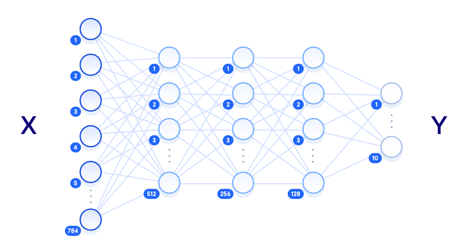
The architecture of the neural network refers to elements such as the number of layers in the network, the number of units in each layer, and how the units are connected between layers. As neural networks are loosely inspired by the workings of the human brain, here the term unit is used to represent what we would biologically think of as a neuron. Like neurons passing signals around the brain, units take some values from previous units as input, perform a computation, and then pass on the new value as output to other units. These units are layered to form the network, starting at a minimum with one layer for inputting values, and one layer to output values. The term hidden layer is used for all of the layers in between the input and output layers, i.e. those “hidden” from the real world.
Different architectures can yield dramatically different results, as the performance can be thought of as a function of the architecture among other things, such as the parameters, the data, and the duration of training.
Add the following lines of code to your file to store the number of units per layer in global variables. This allows us to alter the network architecture in one place, and at the end of the tutorial you can test for yourself how different numbers of layers and units will impact the results of our model:
...
n_input = 784  # input layer (28x28 pixels)
n_hidden1 = 512  # 1st hidden layer
n_hidden2 = 256  # 2nd hidden layer
n_hidden3 = 128  # 3rd hidden layer
n_output = 10  # output layer (0-9 digits)
The following diagram shows a visualization of the architecture we’ve designed, with each layer fully connected to the surrounding layers:
The term “deep neural network” relates to the number of hidden layers, with “shallow” usually meaning just one hidden layer, and “deep” referring to multiple hidden layers. Given enough training data, a shallow neural network with a sufficient number of units should theoretically be able to represent any function that a deep neural network can. But it is often more computationally efficient to use a smaller deep neural network to achieve the same task that would require a shallow network with exponentially more hidden units. Shallow neural networks also often encounter overfitting, where the network essentially memorizes the training data that it has seen, and is not able to generalize the knowledge to new data. This is why deep neural networks are more commonly used: the multiple layers between the raw input data and the output label allow the network to learn features at various levels of abstraction, making the network itself better able to generalize.
Other elements of the neural network that need to be defined here are the hyperparameters. Unlike the parameters that will get updated during training, these values are set initially and remain constant throughout the process. In your file, set the following variables and values:
...
learning_rate = 1e-4
n_iterations = 1000
batch_size = 128
dropout = 0.5
The learning rate represents how much the parameters will adjust at each step of the learning process. These adjustments are a key component of training: after each pass through the network we tune the weights slightly to try and reduce the loss. Larger learning rates can converge faster, but also have the potential to overshoot the optimal values as they are updated. The number of iterations refers to how many times we go through the training step, and the batch size refers to how many training examples we are using at each step. The dropout variable represents a threshold at which we eliminate some units at random. We will be using dropout in our final hidden layer to give each unit a 50% chance of being eliminated at every training step. This helps prevent overfitting.
We have now defined the architecture of our neural network, and the hyperparameters that impact the learning process. The next step is to build the network as a TensorFlow graph.
Step 4 — Building the TensorFlow Graph
To build our network, we will set up the network as a computational graph for TensorFlow to execute. The core concept of TensorFlow is the tensor, a data structure similar to an array or list. initialized, manipulated as they are passed through the graph, and updated through the learning process.
We’ll start by defining three tensors as placeholders, which are tensors that we’ll feed values into later. Add the following to your file:
...
X = tf.placeholder("float", [None, n_input])
Y = tf.placeholder("float", [None, n_output])
keep_prob = tf.placeholder(tf.float32)
The only parameter that needs to be specified at its declaration is the size of the data we will be feeding in. For X we use a shape of [None, 784], where None represents any amount, as we will be feeding in an undefined number of 784-pixel images. The shape of Y is [None, 10] as we will be using it for an undefined number of label outputs, with 10 possible classes. The keep_prob tensor is used to control the dropout rate, and we initialize it as a placeholder rather than an immutable variable because we want to use the same tensor both for training (when dropout is set to 0.5) and testing (when dropout is set to 1.0).
The parameters that the network will update in the training process are the weight and bias values, so for these we need to set an initial value rather than an empty placeholder. These values are essentially where the network does its learning, as they are used in the activation functions of the neurons, representing the strength of the connections between units.
Since the values are optimized during training, we could set them to zero for now. But the initial value actually has a significant impact on the final accuracy of the model. We’ll use random values from a truncated normal distribution for the weights. We want them to be close to zero, so they can adjust in either a positive or negative direction, and slightly different, so they generate different errors. This will ensure that the model learns something useful. Add these lines:
...
weights = {
    'w1': tf.Variable(tf.truncated_normal([n_input, n_hidden1], stddev=0.1)),
    'w2': tf.Variable(tf.truncated_normal([n_hidden1, n_hidden2], stddev=0.1)),
    'w3': tf.Variable(tf.truncated_normal([n_hidden2, n_hidden3], stddev=0.1)),
    'out': tf.Variable(tf.truncated_normal([n_hidden3, n_output], stddev=0.1)),
}
For the bias, we use a small constant value to ensure that the tensors activate in the intial stages and therefore contribute to the propagation. The weights and bias tensors are stored in dictionary objects for ease of access. Add this code to your file to define the biases:
...
biases = {
    'b1': tf.Variable(tf.constant(0.1, shape=[n_hidden1])),
    'b2': tf.Variable(tf.constant(0.1, shape=[n_hidden2])),
    'b3': tf.Variable(tf.constant(0.1, shape=[n_hidden3])),
    'out': tf.Variable(tf.constant(0.1, shape=[n_output]))
}
Next, set up the layers of the network by defining the operations that will manipulate the tensors. Add these lines to your file:
...
layer_1 = tf.add(tf.matmul(X, weights['w1']), biases['b1'])
layer_2 = tf.add(tf.matmul(layer_1, weights['w2']), biases['b2'])
layer_3 = tf.add(tf.matmul(layer_2, weights['w3']), biases['b3'])
layer_drop = tf.nn.dropout(layer_3, keep_prob)
output_layer = tf.matmul(layer_3, weights['out']) + biases['out']
Each hidden layer will execute matrix multiplication on the previous layer’s outputs and the current layer’s weights, and add the bias to these values. At the last hidden layer, we will apply a dropout operation using our keep_prob value of 0.5.
The final step in building the graph is to define the loss function that we want to optimize. A popular choice of loss function in TensorFlow programs is cross-entropy, also known as log-loss, which quantifies the difference between two probability distributions (the predictions and the labels). A perfect classification would result in a cross-entropy of 0, with the loss completely minimized.
We also need to choose the optimization algorithm which will be used to minimize the loss function. A process named gradient descent optimization is a common method for finding the (local) minimum of a function by taking iterative steps along the gradient in a negative (descending) direction. There are several choices of gradient descent optimization algorithms already implemented in TensorFlow, and in this tutorial we will be using the Adam optimizer. This extends upon gradient descent optimization by using momentum to speed up the process through computing an exponentially weighted average of the gradients and using that in the adjustments. Add the following code to your file:
...
cross_entropy = tf.reduce_mean(
    tf.nn.softmax_cross_entropy_with_logits(
        labels=Y, logits=output_layer
        ))
train_step = tf.train.AdamOptimizer(1e-4).minimize(cross_entropy)
We’ve now defined the network and built it out with TensorFlow. The next step is to feed data through the graph to train it, and then test that it has actually learnt something.
Step 5 — Training and Testing
The training process involves feeding the training dataset through the graph and optimizing the loss function. Every time the network iterates through a batch of more training images, it updates the parameters to reduce the loss in order to more accurately predict the digits shown. The testing process involves running our testing dataset through the trained graph, and keeping track of the number of images that are correctly predicted, so that we can calculate the accuracy.
Before starting the training process, we will define our method of evaluating the accuracy so we can print it out on mini-batches of data while we train. These printed statements will allow us to check that from the first iteration to the last, loss decreases and accuracy increases; they will also allow us to track whether or not we have ran enough iterations to reach a consistent and optimal result:
...
correct_pred = tf.equal(tf.argmax(output_layer, 1), tf.argmax(Y, 1))
accuracy = tf.reduce_mean(tf.cast(correct_pred, tf.float32))
In correct_pred, we use the arg_max function to compare which images are being predicted correctly by looking at the output_layer (predictions) and Y (labels), and we use the equal function to return this as a list of Booleans. We can then cast this list to floats and calculate the mean to get a total accuracy score.
We are now ready to initialize a session for running the graph. In this session we will feed the network with our training examples, and once trained, we feed the same graph with new test examples to determine the accuracy of the model. Add the following lines of code to your file:
...
init = tf.global_variables_initializer()
sess = tf.Session()
sess.run(init)
The essence of the training process in deep learning is to optimize the loss function. Here we are aiming to minimize the difference between the predicted labels of the images, and the true labels of the images. The process involves four steps which are repeated for a set number of iterations:
- Propagate values forward through the network
- Compute the loss
- Propagate values backward through the network
- Update the parameters
At each training step, the parameters are adjusted slightly to try and reduce the loss for the next step. As the learning progresses, we should see a reduction in loss, and eventually we can stop training and use the network as a model for testing our new data.
Add this code to the file:
...
# train on mini batches
for i in range(n_iterations):
    batch_x, batch_y = mnist.train.next_batch(batch_size)
    sess.run(train_step, feed_dict={
        X: batch_x, Y: batch_y, keep_prob: dropout
        })

    # print loss and accuracy (per minibatch)
    if i % 100 == 0:
        minibatch_loss, minibatch_accuracy = sess.run(
            [cross_entropy, accuracy],
            feed_dict={X: batch_x, Y: batch_y, keep_prob: 1.0}
            )
        print(
            "Iteration",
            str(i),
            "\t| Loss =",
            str(minibatch_loss),
            "\t| Accuracy =",
            str(minibatch_accuracy)
            )
After 100 iterations of each training step in which we feed a mini-batch of images through the network, we print out the loss and accuracy of that batch. Note that we should not be expecting a decreasing loss and increasing accuracy here, as the values are per batch, not for the entire model. We use mini-batches of images rather than feeding them through individually to speed up the training process and allow the network to see a number of different examples before updating the parameters.
Once the training is complete, we can run the session on the test images. This time we are using a keep_prob dropout rate of 1.0 to ensure all units are active in the testing process.
Add this code to the file:
...
test_accuracy = sess.run(accuracy, feed_dict={X: mnist.test.images, Y: mnist.test.labels, keep_prob: 1.0})
print("\nAccuracy on test set:", test_accuracy)
It’s now time to run our program and see how accurately our neural network can recognize these handwritten digits. Save the main.py file and execute the following command in the terminal to run the script:
- python main.py
You’ll see an output similar to the following, although individual loss and accuracy results may vary slightly:
OutputIteration 0 	| Loss = 3.67079 	| Accuracy = 0.140625
Iteration 100 	| Loss = 0.492122 	| Accuracy = 0.84375
Iteration 200 	| Loss = 0.421595 	| Accuracy = 0.882812
Iteration 300 	| Loss = 0.307726 	| Accuracy = 0.921875
Iteration 400 	| Loss = 0.392948 	| Accuracy = 0.882812
Iteration 500 	| Loss = 0.371461 	| Accuracy = 0.90625
Iteration 600 	| Loss = 0.378425 	| Accuracy = 0.882812
Iteration 700 	| Loss = 0.338605 	| Accuracy = 0.914062
Iteration 800 	| Loss = 0.379697 	| Accuracy = 0.875
Iteration 900 	| Loss = 0.444303 	| Accuracy = 0.90625

Accuracy on test set: 0.9206
To try and improve the accuracy of our model, or to learn more about the impact of tuning hyperparameters, we can test the effect of changing the learning rate, the dropout threshold, the batch size, and the number of iterations. We can also change the number of units in our hidden layers, and change the amount of hidden layers themselves, to see how different architectures increase or decrease the model accuracy.
To demonstrate that the network is actually recognizing the hand-drawn images, let’s test it on a single image of our own.
If you are on a local machine and you would like to use your own hand-drawn number, you can use a graphics editor to create your own 28x28 pixel image of a digit. Otherwise, you can use curl to download the following sample test image to your server or computer:
- curl -O https://raw.githubusercontent.com/do-community/tensorflow-digit-recognition/master/test_img.png
Open the main.py file in your editor and add the following lines of code to the top of the file to import two libraries necessary for image manipulation.
import numpy as np
from PIL import Image
...
Then at the end of the file, add the following line of code to load the test image of the handwritten digit:
...
img = np.invert(Image.open("test_img.png").convert('L')).ravel()
The open function of the Image library loads the test image as a 4D array containing the three RGB color channels and the Alpha transparency. This is not the same representation we used previously when reading in the dataset with TensorFlow, so we’ll need to do some extra work to match the format.
First, we use the convert function with the L parameter to reduce the 4D RGBA representation to one grayscale color channel. We store this as a numpy array and invert it using np.invert, because the current matrix represents black as 0 and white as 255, whereas we need the opposite. Finally, we call ravel to flatten the array.
Now that the image data is structured correctly, we can run a session in the same way as previously, but this time only feeding in the single image for testing.
Add the following code to your file to test the image and print the outputted label.
...
prediction = sess.run(tf.argmax(output_layer, 1), feed_dict={X: [img]})
print ("Prediction for test image:", np.squeeze(prediction))
The np.squeeze function is called on the prediction to return the single integer from the array (i.e. to go from [2] to 2). The resulting output demonstrates that the network has recognized this image as the digit 2.
OutputPrediction for test image: 2
You can try testing the network with more complex images –– digits that look like other digits, for example, or digits that have been drawn poorly or incorrectly –– to see how well it fares.
Conclusion
In this tutorial you successfully trained a neural network to classify the MNIST dataset with around 92% accuracy and tested it on an image of your own. Current state-of-the-art research achieves around 99% on this same problem, using more complex network architectures involving convolutional layers. These use the 2D structure of the image to better represent the contents, unlike our method which flattened all the pixels into one vector of 784 units. You can read more about this topic on the TensorFlow website, and see the research papers detailing the most accurate results on the MNIST website.
Now that you know how to build and train a neural network, you can try and use this implementation on your own data, or test it on other popular datasets such as the Google StreetView House Numbers, or the CIFAR-10 dataset for more general image recognition.
Thanks for learning with the DigitalOcean Community. Check out our offerings for compute, storage, networking, and managed databases.
About the author
Still looking for an answer?
This textbox defaults to using Markdown to format your answer.
You can type !ref in this text area to quickly search our full set of tutorials, documentation & marketplace offerings and insert the link!
img = np.invert(Image.open(“test_img.png”).convert(‘L’)).ravel()
This does not seem to work!!
I was getting this error “ValueError: Cannot feed value of shape (1, 232764) for Tensor ‘Placeholder:0’, which has shape ‘(?, 784)’”
so i added these lines
img = tf.placeholder(tf.float32 , [None ,28 , 28 , 1]) img = tf.reshape(img , [-1 , 784])
now I am getting this error
return array(a, dtype, copy=False, order=order) ValueError: setting an array element with a sequence.
And what’s about non-linear part? It seems that you do only matrix multiplication, so that’s actually equal with linear method.
I think you missed the non-linear activation step. At present this is simply a linear classifier.
the prediction part seems problematic. No matter what image you select it always output 2.
 This work is licensed under a Creative Commons Attribution-NonCommercial- ShareAlike 4.0 International License.
Become a contributor for community
Get paid to write technical tutorials and select a tech-focused charity to receive a matching donation.

DigitalOcean Documentation
Full documentation for every DigitalOcean product.

Resources for startups and AI-native businesses
The Wave has everything you need to know about building a business, from raising funding to marketing your product.
The developer cloud
Scale up as you grow — whether you're running one virtual machine or ten thousand.

Start building today
From GPU-powered inference and Kubernetes to managed databases and storage, get everything you need to build, scale, and deploy intelligent applications.
