By Michelle Morales and Lisa Tagliaferri

Introduction
Python is great for processing data. Often a data set will include multiple variables and many instances, making it hard to get a sense of what is going on. Data visualization is a useful way to help you identify patterns in your data.
For example, say you are a real estate agent and you are trying to understand the relationship between the age of a house and its selling price. If your data included 1 block of 5 houses, it wouldn’t be too difficult to get a sense of what is going on. However, say you wanted to use data from the entire town of 500 houses. Then it would become pretty difficult to understand how age affects price. Visualizing the data, by plotting the selling price versus age, could definitely shed some light on the relationship that exists between the two.
Visualization is a quick and easy way to convey concepts in a universal manner, especially to those who aren’t familiar with your data. Whenever we are working with data, visualization is often a necessary part of the analysis.
We’ll be using the 2D plotting library, matplotlib, which was originally written by John D. Hunter and since then has become a very active open-source development community project. It allows you to generate high quality line plots, scatter plots, histograms, bar charts, and much more. Each plot presents data in a different way and it is often useful to try out different types of plots before settling on the most informative plot for your data. It is good to keep in mind that visualization is a blend of art and science.
Given the importance of visualization, this tutorial will describe how to plot data in Python using matplotlib. We’ll go through generating a scatter plot using a small set of data, adding information such as titles and legends to plots, and customizing plots by changing how plot points look.
When you are finished with this tutorial, you’ll be able to plot data in Python!
Prerequisites
For this tutorial, you should have Python 3 installed, as well as a local programming environment set up on your computer. If this is not the case, you can get set up by following the appropriate installation and set up guide for your operating system.
Step 1 — Importing matplotlib
Before we can begin working in Python, let’s double check that the matplotlib module is installed. In the command line, check for matplotlib by running the following command:
- python -c "import matplotlib"
If matplotlib is installed, this command will complete with no error and we are ready to go. If not, you will receive an error message:
- OutputTraceback (most recent call last): File "<string>", line 1, in <module> ImportError: No module named 'matplolib'
If you receive an error message, download the library using pip:
- pip install matplotlib
Now that matplotlib is installed, we can import it in Python. First, let’s create the script that we’ll be working with in this tutorial: scatter.py. Then, in our script, let’s import matplotlib. Since we’ll only be working with the plotting module (pyplot), let’s specify that when we import it.
import matplotlib.pyplot as plt
We specify the module we wish to import by appending .pyplot to the end of matplotlib. To make it easier to refer to the module in our script, we abbreviate it as plt. Now, we can move on to creating and plotting our data.
Step 2 — Creating Data Points to Plot
In our Python script, let’s create some data to work with. We are working in 2D, so we will need X and Y coordinates for each of our data points.
To best understand how matplotlib works, we’ll associate our data with a possible real-life scenario. Let’s pretend we are owners of a coffee shop and we’re interested in the relationship between the average weather throughout the year and the total number of purchases of iced coffee. Our X variable will be the total number of iced coffees sold per month, and our Y variable will be the average temperature in Fahrenheit for each month.
In our Python script, we’ll create two list variables: X (total iced coffees sold) and Y (average temperature). Each item in our respective lists will represent data from each month (January to December). For example, in January the average temperature was 32 degrees Fahrenheit and the coffee shop sold 590 iced coffees.
import matplotlib.pyplot as plt

X = [590,540,740,130,810,300,320,230,470,620,770,250]
Y = [32,36,39,52,61,72,77,75,68,57,48,48]
Now that we have our data, we can begin plotting.
Step 3 — Plotting Data
Scatter plots are great for determining the relationship between two variables, so we’ll use this graph type for our example. To create a scatter plot using matplotlib, we will use the scatter() function. The function requires two arguments, which represent the X and Y coordinate values.
import matplotlib.pyplot as plt

X = [590,540,740,130,810,300,320,230,470,620,770,250]
Y = [32,36,39,52,61,72,77,75,68,57,48,48]

plt.scatter(X,Y)
plt.show()
Every time we create a plot we must also specify that we want the plot to show by using plt.show().
Before moving on, let’s check that our script is working. Save the script and run it via the command line:
- python scatter.py
If everything went well, a window should have launched displaying the plot, like so:
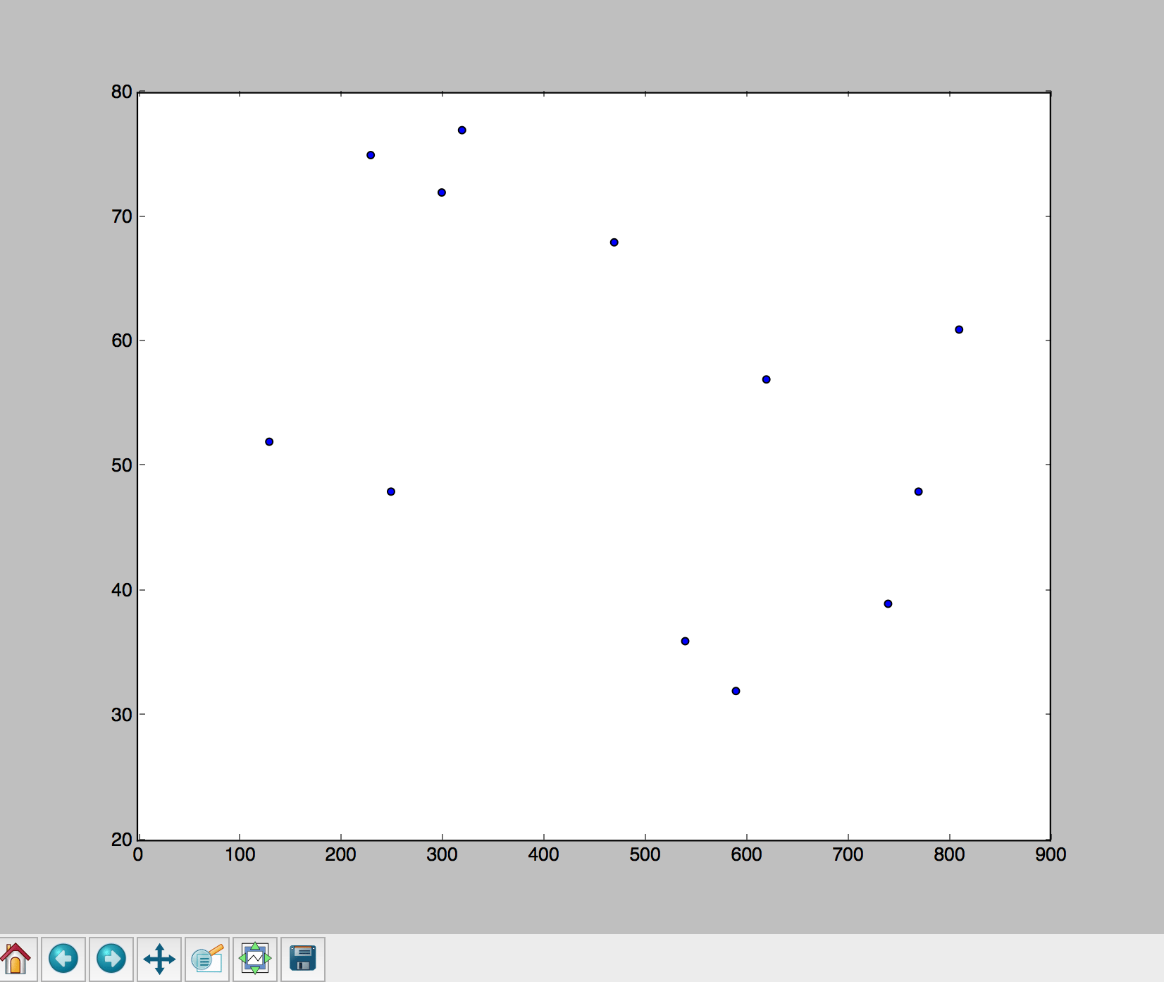
This window is great for viewing data; it’s interactive and includes several functionalities, such as hovering to display labels and coordinates, zooming in or out, and saving.
Step 4 — Adding Titles and Labels
Now that we know our script is working properly, we can begin adding information to our plot. To make it clear what our data represents, let’s include a title as well as labels for each axis.
We’ll begin by adding a title. We add the title before the plt.show() line in our script.
import matplotlib.pyplot as plt
X = [590,540,740,130,810,300,320,230,470,620,770,250]
Y = [32,36,39,52,61,72,77,75,68,57,48,48]
plt.scatter(X,Y)
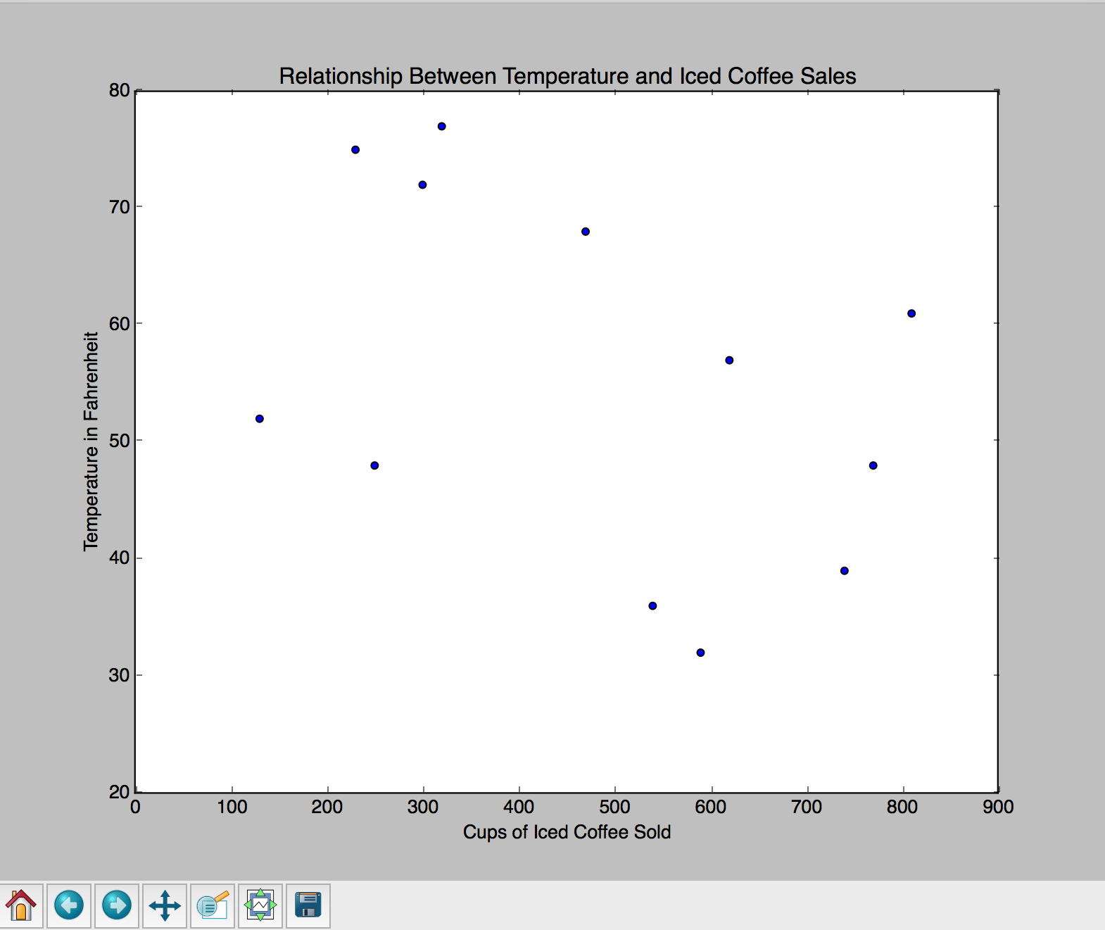
plt.title('Relationship Between Temperature and Iced Coffee Sales')
plt.show()
Next, add labels for the axes right below the plt.title line:
...
plt.xlabel('Cups of Iced Coffee Sold')
plt.ylabel('Temperature in Fahrenheit')
...
If we save our script and run it again, we should now have an updated plot that is more informative. Our updated plot should look something like this:
Step 5 — Customizing a Plot
Every data set we work with will be unique and it’s important to be able to customize how we would like to display our information. Remember visualization is also an art, so get creative with it! matplotlib includes many customization features, such as different colors, point symbols, and sizing. Depending on our needs, we may want to play around with different scales, using different ranges for our axes. We can change the default parameters by designating new ranges for the axes, like so:
import matplotlib.pyplot as plt

X = [590,540,740,130,810,300,320,230,470,620,770,250]
Y = [32,36,39,52,61,72,77,75,68,57,48,48]

plt.scatter(X,Y)

plt.xlim(0,1000)
plt.ylim(0,100)

plt.title('Relationship Between Temperature and Iced Coffee Sales')

plt.show()
...
The points from the original plot did look a bit small and blue may not be the color we want. Perhaps we want triangles instead of circles for our points. If we want to change the actual color/size/shape of the points, we have to make these changes in the initial plt.scatter() call. We’ll change the following parameters:
s: size of point, default = 20c: color, sequence, or sequence of color, default = ‘b’marker: point symbol, default = ‘o’
Possible markers include a number of different shapes, such as diamonds, hexagons, stars, and so on. Color choices include, but are not limited to blue, green, red, and magenta. It is also possible to provide an HTML hex string for color. See matplotlib’s documentation for comprehensive lists of possible markers and colors.
To make our plot easier to read, let’s triple the size of the points (s=60), change the color to red (c='r'), and change the symbol to a triangle (marker='^'). We’ll modify the plt.scatter() function:
plt.scatter(X, Y, s=60, c='red', marker='^')
Before running our updated script, we can double check that our code is right. The updated script for the custom plot should look something like this:
import matplotlib.pyplot as plt


X = [590,540,740,130,810,300,320,230,470,620,770,250]
Y = [32,36,39,52,61,72,77,75,68,57,48,48]

#scatter plot
plt.scatter(X, Y, s=60, c='red', marker='^')

#change axes ranges
plt.xlim(0,1000)
plt.ylim(0,100)

#add title
plt.title('Relationship Between Temperature and Iced Coffee Sales')

#add x and y labels
plt.xlabel('Cups of Iced Coffee Sold')
plt.ylabel('Temperature in Fahrenheit')

#show plot
plt.show()
Don’t forget to save your script before moving on to Step 6.
Step 6 — Saving a Plot
Now that we have finished our code, let’s run it to see our new customized plot.
- python scatter.py
A window should now open displaying our plot:
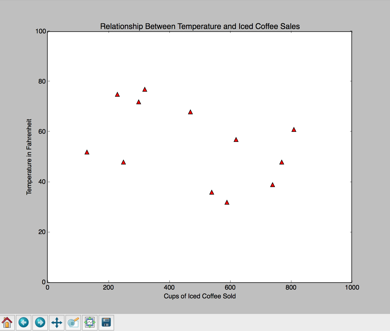
Next, save the plot by clicking on the save button, which is the disk icon located on the bottom toolbar. Keep in mind the image will be saved as a PNG instead of an interactive graph. You now have your very own customized scatter plot, congratulations!
Conclusion
In this tutorial, you learned how to plot data using matplotlib in Python. You can now visualize data and customize plots.
To continue practicing with matplotlib, you can follow our guide on “How To Graph Word Frequency Using matplotlib with Python 3.”
Thanks for learning with the DigitalOcean Community. Check out our offerings for compute, storage, networking, and managed databases.
About the author(s)
Community and Developer Education expert. Former Senior Manager, Community at DigitalOcean. Focused on topics including Ubuntu 22.04, Ubuntu 20.04, Python, Django, and more.
Still looking for an answer?
This textbox defaults to using Markdown to format your answer.
You can type !ref in this text area to quickly search our full set of tutorials, documentation & marketplace offerings and insert the link!
Wow! That’s absolutely awesome! I like that, I want to become a good Data Scientist and I’m reading and applying your “How to Code in Python 3” book as e-book. The book and tutorials are veri good. Thanks for these service l, seriously…
how can i get my system time on x axis . currently i am using “x.append(time())” i am not getting plots in hh::mm format. can you please help for getting time in 24 hour format
 This work is licensed under a Creative Commons Attribution-NonCommercial- ShareAlike 4.0 International License.
Become a contributor for community
Get paid to write technical tutorials and select a tech-focused charity to receive a matching donation.

DigitalOcean Documentation
Full documentation for every DigitalOcean product.

Resources for startups and AI-native businesses
The Wave has everything you need to know about building a business, from raising funding to marketing your product.
The developer cloud
Scale up as you grow — whether you're running one virtual machine or ten thousand.

Start building today
From GPU-powered inference and Kubernetes to managed databases and storage, get everything you need to build, scale, and deploy intelligent applications.
