By Julius Volz and Tammy Fox

An Article from Prometheus co-creator Julius Volz
Introduction
Prometheus is an open source monitoring system and time series database. In How To Query Prometheus on Ubuntu 14.04 Part 1, we set up three demo service instances exposing synthetic metrics to a Prometheus server. Using these metrics, we then learned how use the Prometheus query language to select and filter time series, how to aggregate over dimensions, as well as how to compute rates and derivatives.
In the second part of this tutorial, we will build on the setup from the first part and learn more advanced querying techniques and patterns. After this tutorial, you will know how to apply value-based filtering, set operations, histograms, and more.
Prerequisites
This tutorial is based on the setup outlined in How To Query Prometheus on Ubuntu 14.04 Part 1. At a minimum, you will need to follow Steps 1 and Step 2 from that tutorial to set up a Prometheus server and three monitored demo service instances. However, we will also build on the query language techniques explained in the first part and thus recommend working through it entirely.
Step 1 — Filtering by Value and Using Thresholds
In this section, we will learn how to filter returned time series based on their value.
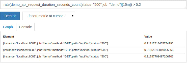
The most common use for value-based filtering is for simple numeric alert thresholds. For example, we may want to find HTTP paths that have a higher total 500-status request rate than 0.2 per second, as averaged over the last 15 minutes. To do this, we simply query for all 500-status request rates and then append a > 0.2 filter operator at the end of the expression:
rate(demo_api_request_duration_seconds_count{status="500",job="demo"}[15m]) > 0.2
In the Console view, the result should look like this:
However, as with binary arithmetic, Prometheus does not only support filtering by a single scalar number. You can also filter one set of time series based on another set of series. Again, elements are matched up by their label sets, and the filter operator is applied between matching elements. Only the elements from the left-hand side that match an element on the right-hand side and that pass the filter become part of the output. The on(<labels>), group_left(<labels>), group_right(<labels>) clauses work the same way here as in arithmetic operators.
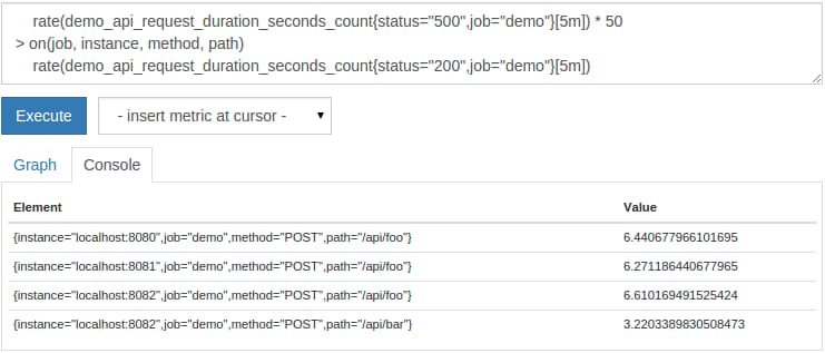
For example, we could select the 500-status rate for any job, instance, method, and path combinations for which the 200-status rate is not at least 50 times higher than the 500-status rate like this:
    rate(demo_api_request_duration_seconds_count{status="500",job="demo"}[5m]) * 50
> on(job, instance, method, path)
    rate(demo_api_request_duration_seconds_count{status="200",job="demo"}[5m])
This will look like the following:
Besides >, Prometheus also supports the usual >=, <=, <, !=, and == comparison operators for use in filtering.
We now know how to filter a set of time series either based on a single numeric value or based on another set of time series values with matching labels.
Step 2 — Using Set Operators
In this section, you will learn how to use Prometheus’s set operators to correlate sets of time series with each other.
Often you want to filter one set of time series based on another set. For this, Prometheus provides the and set operator. For every series on the left side of the operator, it tries to find a series on the right side with the same labels. If a match is found, the left-hand-side series becomes part of the output. If no matching series exists on the right, the series is omitted from the output.
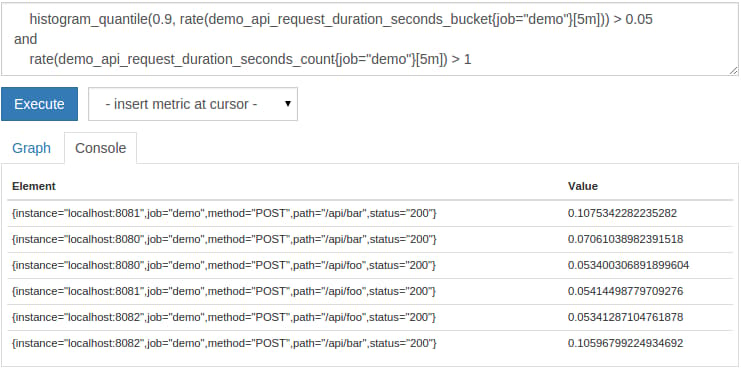
For example, you may want select any HTTP endpoints that have a 90th percentile latency higher than 50ms (0.05s) but only for the dimensional combinations that receive more than one request per second. We will use the histogram_quantile() function for the percentile calculation here. We will explain in the next section exactly this functions works. For now, it only matters that it calculates the 90th percentile latency for each sub-dimension. To filter the resulting bad latencies and retain only those that receive more than one request per second, we can query for:
    histogram_quantile(0.9, rate(demo_api_request_duration_seconds_bucket{job="demo"}[5m])) > 0.05
and
    rate(demo_api_request_duration_seconds_count{job="demo"}[5m]) > 1
Instead of taking the intersection, sometimes you want to build the union out of two sets of time series. Prometheus provides the or set operator for this. It results in the series of the left-hand side of the operation, as well as any series from the right-hand side which don’t have matching label sets on the left. For example, to list all request rates which are either below 10 or above 30, query for:
    rate(demo_api_request_duration_seconds_count{job="demo"}[5m]) < 10
or
    rate(demo_api_request_duration_seconds_count{job="demo"}[5m]) > 30
The result will look like this in a graph:
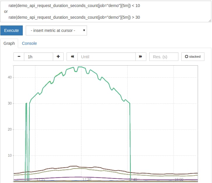
As you can see, using value filters and set operations in graphs can lead to time series appearing and disappearing within the same graph, depending on whether they match a filter or not at any time step along the graph. Generally, using this kind of filter logic is recommended only for alerting rules.
You now know how to build intersections and unions out of labeled time series.
Step 3 — Working with Histograms
In this section, we will learn how to interpret histogram metrics and how to calculate quantiles (a generalized form of percentiles) from them.
Prometheus supports histogram metrics, which allow a service to record the distribution of a series of values. Histograms usually track measurements like request latencies or response sizes, but can fundamentally track any value that fluctuates in magnitude according to some distribution. Prometheus histograms sample data on the client-side, meaning that they count observed values using a number of configurable (e.g. latency) buckets and then expose those buckets as individual time series.
Internally, histograms are implemented as a group of time series that each represent the count for a given bucket (e.g. “requests under 10ms”, “requests under 25ms”, “requests under 50ms”, and so on). The bucket counters are cumulative, meaning that buckets for larger values include the counts for all lower-valued buckets. On each time series that is part of a histogram, the corresponding bucket is indicated by the special le (less-than-or-equal) label. This adds an additional dimension to any existing dimensions you are already tracking.
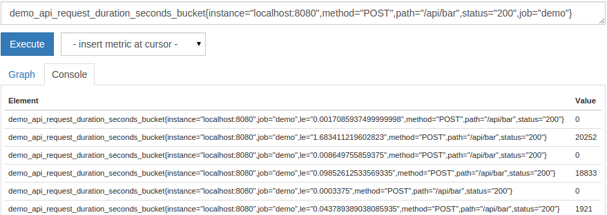
For example, our demo service exports a histogram demo_api_request_duration_seconds_bucket that tracks the distribution of API request durations. Since this histogram exports 26 buckets per tracked sub-dimension, this metric has a lot of time series. Let’s first look at the raw histogram only for one type of request, from one instance:
demo_api_request_duration_seconds_bucket{instance="localhost:8080",method="POST",path="/api/bar",status="200",job="demo"}
You should see 26 series that each represent one observation bucket, identified by the le label:
A histogram can help you answer questions like “How many of my requests take longer than 100ms to complete?” (provided the histogram has a bucket configured that has a 100ms boundary). On the other hand, you often would like to answer a related question like “What is the latency at which 99% of my queries complete?”. If your histogram buckets are fine-grained enough, you can calculate this using the histogram_quantile() function. This function expects a histogram metric (a group of series with le bucket labels) as its input and outputs corresponding quantiles. In contrast to percentiles, which range from the 0th to the 100th percentile, the target quantile specification that the histogram_quantile() function expects as an input ranges from 0 to 1 (so the 90th percentile would correspond to a quantile of 0.9).
For example, we could attempt to calculate the 90th percentile API latency over all time for all dimensions like this:
# BAD!
histogram_quantile(0.9, demo_api_request_duration_seconds_bucket{job="demo"})
This is not very useful or reliable. The bucket counters reset when individual service instances are restarted, and you usually want to see what the latency is “now” (for example, as measured over the last 5 minutes), rather than over the entire time of the metric. You can achieve this by applying a rate() function to the underlying histogram bucket counters, which both deals with counter resets and also only considers each bucket’s rate of increase over the specified time window.
Calculate the 90th percentile API latency over the last 5 minutes like this:
# GOOD!
histogram_quantile(0.9, rate(demo_api_request_duration_seconds_bucket{job="demo"}[5m]))
This is much better and will look like this:
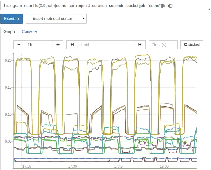
However, this shows you the 90th percentile for every sub-dimension (job, instance, path, method, and status). Again, we might not be interested in all of those dimensions and want to aggregate some of them away. Fortunately, Prometheus’s sum aggregation operator can be composed together with the histogram_quantile() function to allow us to aggregate over dimensions during query time!
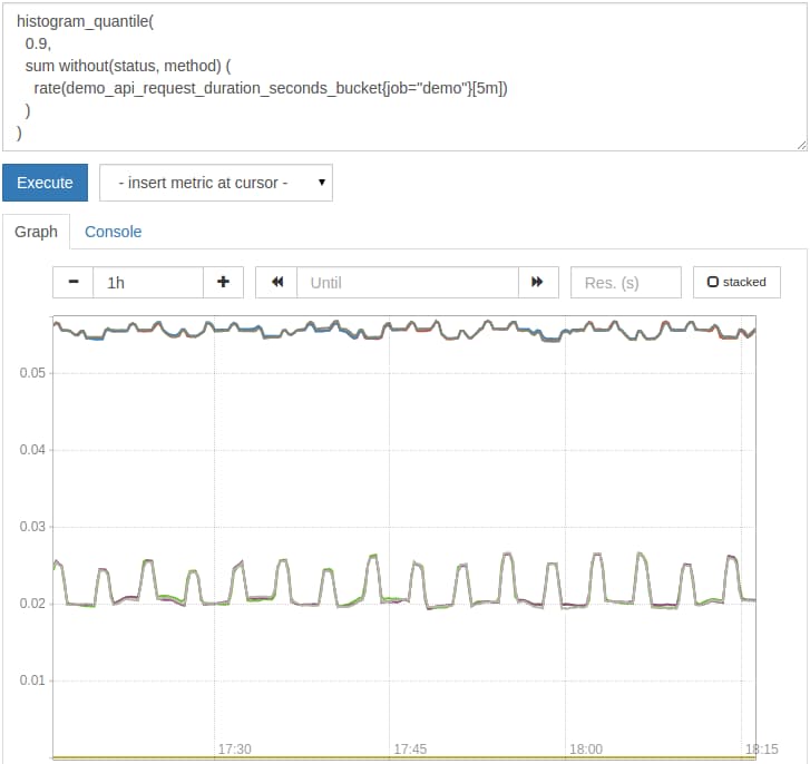
The following query calculates the 90th percentile latency, but splits the result only by job, instance and path dimensions:
histogram_quantile(
  0.9,
  sum without(status, method) (
    rate(demo_api_request_duration_seconds_bucket{job="demo"}[5m])
  )
)
Note: Always preserve the le bucket label in any aggregations before applying the histogram_quantile() function. This ensures that it can still operate on groups of buckets and calculate quantiles from them.
The graph will now look like this:
Computing quantiles from histograms always introduces some amount of statistical error. This error depends on your bucket sizes, the distribution of the observed values, as well as the target quantiles you want to calculate. To learn more about this, read about Errors of quantile estimation in the Prometheus documentation.
You now know how to interpret histogram metrics and how to calculate quantiles from them for different time ranges, while also aggregating over some dimensions on the fly.
Step 4 — Working with Timestamp Metrics
In this section, we will learn how to make use of metrics that contain timestamps.
Components in the Prometheus ecosystem frequently expose timestamps. For example, this might be the last time that a batch job completed successfully, the last time a configuration file was reloaded successfully, or when a machine was booted. By convention, times are represented as Unix timestamps in seconds since January 1, 1970 UTC.
For example, the demo service exposes the last time when a simulated batch job succeeded:
demo_batch_last_success_timestamp_seconds{job="demo"}
This batch job is simulated to be run once per minute, but fails in 25% of all attempts. In the failure case, the demo_batch_last_success_timestamp_seconds metric keeps its last value until another successful run occurs.
If you graph the raw timestamp, it will look somewhat like this:
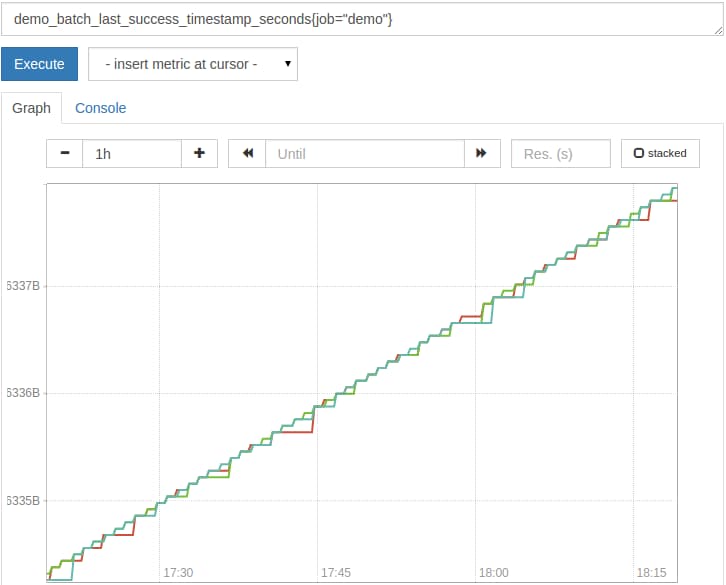
As you can see, the raw timestamp value is usually not very useful by itself. Instead, you often want to know how old the timestamp value is. A common pattern is to subtract the timestamp in the metric from the current time, as provided by the time() function:
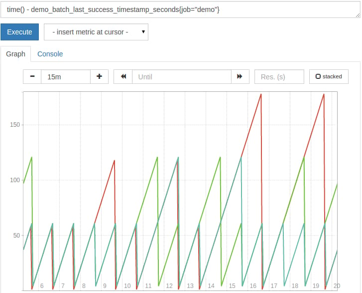
time() - demo_batch_last_success_timestamp_seconds{job="demo"}
This yields the time in seconds since the last successful batch job run:
If you wanted to convert this age from seconds into hours, you could divide the result by 3600:
(time() - demo_batch_last_success_timestamp_seconds{job="demo"}) / 3600
An expression like this is useful for both graphing and alerting. When visualizing the timestamp age like above, you receive a sawtooth graph, with linearly increasing lines and regular resets to 0 when the batch job completes successfully. If a sawtooth spike gets too large, this indicates a batch job that has not completed in a long time. You can also alert on this by adding a > threshold filter to the expression and alerting on the resulting time series (though we will not cover alerting rules in this tutorial).
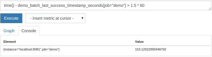
To simply list instances for which the batch job has not completed in the last 1.5 minutes, you can run the following query:
time() - demo_batch_last_success_timestamp_seconds{job="demo"} > 1.5 * 60
You now know how to transform raw timestamp metrics into relative ages, which is helpful both for graphing and alerting.
Step 5 — Sorting and Using the topk / bottomk Functions
In this step, you will learn how to sort query output or select only the biggest or smallest values of a set of series.
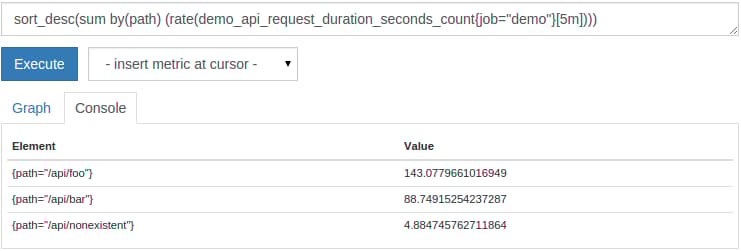
In the tabular Console view, it is often useful to sort the output series by their value. You can achieve this by using the sort() (ascending sort) and sort_desc() (descending sort) functions. For example, to show per-path request rates sorted by their value, from highest to lowest, you can query for:
sort_desc(sum by(path) (rate(demo_api_request_duration_seconds_count{job="demo"}[5m])))
The sorted output will look like this:
Or maybe you are not even interested in showing all series at all, but only the K largest or smallest series. For this, Prometheus provides the topk() and bottomk() functions. They each take a K value (how many series you want to select) and an arbitrary expression that returns a set of time series that should be filtered. For example, to show only the top three request rates per path and method, you can query for:
topk(3, sum by(path, method) (rate(demo_api_request_duration_seconds_count{job="demo"}[5m])))
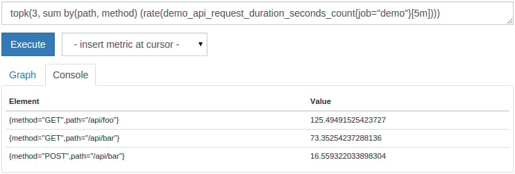
While sorting is only useful in the Console view, topk() and bottomk() may also be useful in graphs. Just be aware that the output will not show the top or bottom K series as averaged over the entire graph time range — instead, the output will re-compute the K top or bottom output series for every resolution step along the graph. Thus, your top or bottom K series can actually vary over the range of the graph, and your graph may show more than K series in total.
We now learned how to sort or only select the K largest or smallest series.
Step 6 — Inspecting the Health of Scraped Instances
In this step, we will learn how inspect the scrape health of our instances over time.
To make the section more interesting, let’s terminate the first of your three backgrounded demo service instances (the one listening on port 8080):
- pkill -f -- -listen-address=:8080
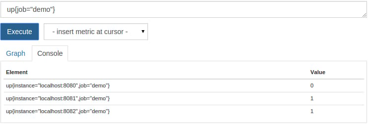
Whenever Prometheus scrapes a target, it stores a synthetic sample with the metric name up and the job and instance labels of the scraped instance. If the scrape was successful, the value of the sample is set to 1. It is set to 0 if the scrape fails. Thus, we can easily query which instances are currently “up” or “down”:
up{job="demo"}
This should now show one instance as down:
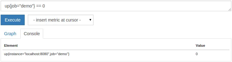
To show only down instances, you could filter for the value 0:
up{job="demo"} == 0
You should now only see the instance you terminated:
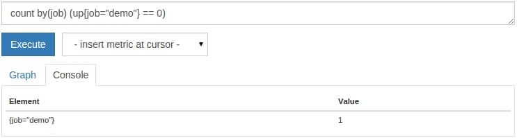
Or, to get the total count of down instances:
count by(job) (up{job="demo"} == 0)
This will show you a count of 1:
These kinds of queries are useful for basic scrape health alerting.
Note: When there are no down instances, this query returns an empty result instead of a single output series with a count of 0. This is because count() is an aggregation operator that expects a set of dimensional time series as its input and can group the output series according to a by or without clause. Any output groups could only be based on existing input series - if there are no input series at all, no output is produced.
You now know how to query for instance health state.
Conclusion
In this tutorial, we built on the progress of How To Query Prometheus on Ubuntu 14.04 Part 1 and covered more advanced query techniques and patterns. We learned how to filter series based on their value, compute quantiles from histograms, deal with timestamp-based metrics, and more.
While these tutorials cannot cover all possible querying use cases, we hope that the example queries will be useful for you when building real-world queries, dashboards, and alerts with Prometheus. For more details about Prometheus’s query language, see the Prometheus query language documentation.
Thanks for learning with the DigitalOcean Community. Check out our offerings for compute, storage, networking, and managed databases.
Tutorial Series: How To Query Prometheus
We will learn how to query Prometheus 1.3.1. In order to have fitting example data to work with, we will set up three identical demo service instances that export synthetic metrics of various kinds. We will then set up a Prometheus server to scrape and store those metrics. Using the example metrics, we will then learn how to query Prometheus, beginning with simple queries and moving on to more advanced ones.
Browse Series: 2 tutorials
About the author(s)
Co-creator of the Prometheus monitoring system. Infrastructure software developer.
Technical Editor, DigitalOcean
Still looking for an answer?
This textbox defaults to using Markdown to format your answer.
You can type !ref in this text area to quickly search our full set of tutorials, documentation & marketplace offerings and insert the link!
 This work is licensed under a Creative Commons Attribution-NonCommercial- ShareAlike 4.0 International License.
Become a contributor for community
Get paid to write technical tutorials and select a tech-focused charity to receive a matching donation.

DigitalOcean Documentation
Full documentation for every DigitalOcean product.

Resources for startups and AI-native businesses
The Wave has everything you need to know about building a business, from raising funding to marketing your product.
The developer cloud
Scale up as you grow — whether you're running one virtual machine or ten thousand.

Start building today
From GPU-powered inference and Kubernetes to managed databases and storage, get everything you need to build, scale, and deploy intelligent applications.
