By Julius Volz and Hazel Virdó

An Article from Prometheus co-creator Julius Volz
Introduction
Prometheus is an open source monitoring system and time series database. One of Prometheus’s most important aspects is its multi-dimensional data model along with the accompanying query language. This query language allows you to slice and dice your dimensional data to answer operational questions in an ad-hoc way, display trends in dashboards, or generate alerts about failures in your systems.
In this tutorial, we will learn how to query Prometheus 1.3.1. In order to have fitting example data to work with, we will set up three identical demo service instances that export synthetic metrics of various kinds. We will then set up a Prometheus server to scrape and store those metrics. Using the example metrics, we will then learn how to query Prometheus, beginning with simple queries and moving on to more advanced ones.
After this tutorial, you will know how to select and filter time series based on their dimensions, aggregate and transform time series, as well as how to do arithmetics between different metrics. In a follow-up tutorial, How To Query Prometheus on Ubuntu 14.04 Part 2, we will build on the knowledge from this tutorial to cover more advanced querying use cases.
Prerequisites
To follow this tutorial, you will need:
- One Ubuntu 14.04 server set up by following the initial server setup guide for Ubuntu 14.04, including a sudo non-root user.
Step 1 — Installing Prometheus
In this step, we will download, configure, and run a Prometheus server to scrape three (not yet running) demo service instances.
First, download Prometheus:
- wget https://github.com/prometheus/prometheus/releases/download/v1.3.1/prometheus-1.3.1.linux-amd64.tar.gz
Extract the tarball:
- tar xvfz prometheus-1.3.1.linux-amd64.tar.gz
Create a minimal Prometheus configuration file on the host filesystem at ~/prometheus.yml:
- nano ~/prometheus.yml
Add the following contents to the file:
# Scrape the three demo service instances every 5 seconds.
global:
  scrape_interval: 5s

scrape_configs:
  - job_name: 'demo'
    static_configs:
      - targets:
        - 'localhost:8080'
        - 'localhost:8081'
        - 'localhost:8082'
Save and exit nano.
This example configuration makes Prometheus scrape the demo instances. Prometheus works with a pull model, which is why it needs to be configured to know about the endpoints to pull metrics from. The demo instances are not yet running but will run on port 8080, 8081, and 8082 later.
Start Prometheus using nohup and as a background process:
- nohup ./prometheus-1.3.1.linux-amd64/prometheus -storage.local.memory-chunks=10000 &
The nohup at the beginning of command sends the output to the file ~/nohup.out instead of stdout. The & at the end of the command will allow the process to keep running in the background while giving you your prompt back for additional commands. To bring the process back to the foreground (i.e., back to the running process of the terminal), use the command fg at the same terminal.
If all goes well, in the ~/nohup.out file, you should see output similar to the following:
time="2016-11-23T03:10:33Z" level=info msg="Starting prometheus (version=1.3.1, branch=master, revision=be476954e80349cb7ec3ba6a3247cd712189dfcb)" source="main.go:75"
time="2016-11-23T03:10:33Z" level=info msg="Build context (go=go1.7.3, user=root@37f0aa346b26, date=20161104-20:24:03)" source="main.go:76"
time="2016-11-23T03:10:33Z" level=info msg="Loading configuration file prometheus.yml" source="main.go:247"
time="2016-11-23T03:10:33Z" level=info msg="Loading series map and head chunks..." source="storage.go:354"
time="2016-11-23T03:10:33Z" level=info msg="0 series loaded." source="storage.go:359"
time="2016-11-23T03:10:33Z" level=warning msg="No AlertManagers configured, not dispatching any alerts" source="notifier.go:176"
time="2016-11-23T03:10:33Z" level=info msg="Starting target manager..." source="targetmanager.go:76"
time="2016-11-23T03:10:33Z" level=info msg="Listening on :9090" source="web.go:240"
In another terminal, you can monitor the contents of this file with the command tail -f ~/nohup.out. As content is written to the file, it will be displayed to the terminal.
By default, Prometheus will load its configuration from prometheus.yml (which we just created) and store its metrics data in ./data in the current working directory.
The -storage.local.memory-chunks flag adjusts Prometheus’s memory usage to the host system’s very small amount of RAM (only 512MB) and small number of stored time series in this tutorial.
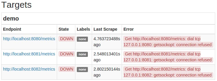
You should now be able to reach your Prometheus server at http://your_server_ip:9090/. Verify that it is configured to collect metrics from the three demo instances by heading to http://your_server_ip:9090/status and locating the three target endpoints for the demo job in the Targets section. The State column for all three targets should show the the target’s state as DOWN since the demo instances have not been started yet and thus cannot be scraped:
Step 2 — Installing the Demo Instances
In this section, we will install and run the three demo service instances.
Download the demo service:
- wget https://github.com/juliusv/prometheus_demo_service/releases/download/0.0.4/prometheus_demo_service-0.0.4.linux-amd64.tar.gz
Extract it:
- tar xvfz prometheus_demo_service-0.0.4.linux-amd64.tar.gz
Run the demo service three times on separate ports:
- ./prometheus_demo_service -listen-address=:8080 &
- ./prometheus_demo_service -listen-address=:8081 &
- ./prometheus_demo_service -listen-address=:8082 &
The & starts the demo services in the background. They will not log anything, but they will expose Prometheus metrics on the /metrics HTTP endpoint on their respective ports.
These demo services export synthetic metrics about several simulated subsystems. These are:
- An HTTP API server that exposes request counts and latencies (keyed by path, method, and response status code)
- A periodic batch job that exposes the timestamp of its last successful run and the number of processed bytes
- Synthetic metrics about the number of CPUs and their usage
- Synthetic metrics about the total size of a disk and its usage
The individual metrics are introduced in the querying examples in later sections.
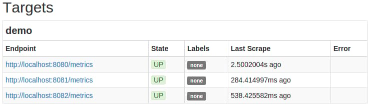
The Prometheus server should now automatically start scraping your three demo instances. Head to your Prometheus server’s status page at http://your_server_ip:9090/status and verify that the targets for the demo job are now showing an UP state:
Step 3 — Using the Query Browser
In this step, we will familiarize ourselves with Prometheus’s built-in querying and graphing web interface. While this interface is great for ad-hoc data exploration and learning about Prometheus’s query language, it is not suitable for building persistent dashboards and does not support advanced visualization features. For building dashboards, see the example How To Add a Prometheus Dashboard to Grafana.
Go to http://your_server_ip:9090/graph on your Prometheus server. It should look like this:
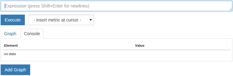
As you can see, there are two tabs: Graph and Console. Prometheus lets you query data in two different modes:
- The Console tab allows you to evaluate a query expression at the current time. After running the query, a table will show the current value of each result time series (one table row per output series).
- The Graph tab allows you to graph a query expression over a specified range of time.
Since Prometheus can scale to millions of time series, it is possible to build very expensive queries (think of this as similar to selecting all rows from a large table in a SQL database). To avoid queries that time out or overload your server, it is recommended to start exploring and building queries in the Console view first rather than graphing them right away. Evaluating a potentially costly query at a single point in time will use far fewer resources than trying to graph the same query over a range of time.
Once you have sufficiently narrowed down a query (in terms of series it selects for loading, computations it needs to perform, and the number of output time series), you can then switch to the Graph tab to show the evaluated expression over time. Knowing when a query is cheap enough to be graphed is not an exact science and depends on your data, your latency requirements, and the power of the machine you are running your Prometheus server on. You will get a feeling for this over time.
Since our test Prometheus server will not scrape a lot of data, we will not actually be able to formulate any costly queries in this tutorial. Any example queries may be viewed both in the Graph and the Console view without risk.
To reduce or increase the graph time range, click the - or + buttons. To move the end time of the graph, press the << or >> buttons. You may stack a graph by activating the stacked checkbox. Finally, the Res. (s) input allows you to specify a custom query resolution (not needed in this tutorial).
Step 4 — Performing Simple Time Series Queries
Before we start querying, let’s quickly review Prometheus’s data model and terminology. Prometheus fundamentally stores all data as time series. Each time series is identified by a metric name, as well as a set of key-value pairs that Prometheus calls labels. The metric name indicates the overall aspect of a system that is being measured (for example, the number of handled HTTP requests since process startup, http_requests_total). Labels serve to differentiate sub-dimensions of a metric such as the HTTP method (e.g. method="POST") or the path (e.g. path="/api/foo"). Finally, a sequence of samples forms the actual data for a series. Each sample consists of a timestamp and a value, where timestamps have millisecond precision and values are always 64-bit floating point values.
The simplest query we can formulate returns all series that have a given metric name. For example, the demo service exports a metric demo_api_request_duration_seconds_count that represents the number of synthetic API HTTP requests handled by the dummy service. You may be wondering why the metric name contains the string duration_seconds. This is because this counter is part of a larger histogram metric named demo_api_request_duration_seconds which primarily tracks a distribution of request durations but also exposes a total count of tracked requests (suffixed by _count here) as a useful by-product.
Make sure the Console query tab is selected, enter the following query in the text field at the top of the page, and click the Execute button to perform the query:
demo_api_request_duration_seconds_count
Since Prometheus is monitoring three service instances, you should see a tabular output containing 27 resulting time series with this metric name, one for each tracked service instance, path, HTTP method, and HTTP status code. Besides labels set by the service instances themselves (method, path, and status), the series will have appropriate job and instance labels that distinguish the different service instances from each other. Prometheus attaches these labels automatically when storing time series from scraped targets. The output should look like this:
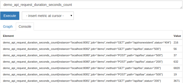
The numeric value shown in the right-hand-side table column is the current value of each time series. Feel free to graph the output (click the Graph tab and click Execute again) for this and subsequent queries to see how the values develop over time.
We can now add label matchers to limit the returned series based on their labels. Label matchers directly follow the metric name in curly braces. In the simplest form, they filter for series that have an exact value for a given label. For example, this query will only show the request count for any GET requests:
demo_api_request_duration_seconds_count{method="GET"}
Matchers may be combined using commas. For example, we could additionally filter for metrics only from instance localhost:8080 and the job demo:
demo_api_request_duration_seconds_count{instance="localhost:8080",method="GET",job="demo"}
The result will look like this:
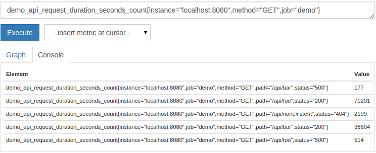
When combining multiple matchers, all of them need to match to select a series. The expression above returns only API request counts for the service instance running on port 8080 and where the HTTP method was GET. We also ensure that we only select metrics belonging to the demo job.
Note: It is recommended to always specify the job label when selecting time series. This ensures that you are not accidentally selecting metrics with the same name from a different job (unless, of course, that is really your goal!). Although we only monitor one job in this tutorial, we will still select by the job name in most of the following examples to emphasize the importance of this practice.
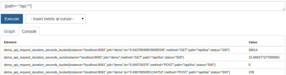
Besides equality matching, Prometheus supports non-equality matching (!=), regular-expression matching (=~), as well as negative regular-expression matching (!~). It is also possible to omit the metric name completely and only query using label matchers. For example, to list all series (no matter which metric name or job) where the path label starts with /api, you can run this query:
{path=~"/api.*"}
The above regular expression needs to end with .* since regular expressions always match a full string in Prometheus.
The resulting time series will be a mix of series with different metric names:
You now know how to select time series by their metric names, as well as by a combination of their label values.
Step 5 — Calculating Rates and Other Derivatives
In this section, we will learn how to calculate rates or deltas of a metric over time.
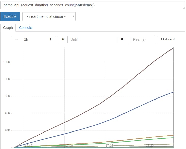
One of the most frequent functions you will use in Prometheus is rate(). Instead of calculating event rates directly in the instrumented service, in Prometheus it is common to track events using raw counters and to let the Prometheus server calculate rates ad-hoc during query time (this has a number of advantages, such as not losing rate spikes between scrapes, as well as being able to choose dynamic averaging windows at query time). Counters start at 0 when a monitored service starts and get continuously incremented over the service process’s life time. Occasionally, when a monitored process restarts, its counters reset to 0 and begin climbing again from there. Graphing raw counters is usually not very useful, as you will only see an ever-increasing line with occasional resets. You can see that by graphing the demo service’s API request counts:
demo_api_request_duration_seconds_count{job="demo"}
It will look somewhat like this:
To make counters useful, we can use the rate() function to calculate their per-second rate of increase. We need to tell rate() over which time window to average the rate by providing a range selector after the series matcher (like [5m]). For example, to compute the per-second increase of the above counter metric, as averaged over the last five minutes, graph the following query:
rate(demo_api_request_duration_seconds_count{job="demo"}[5m])
The result is now much more useful:
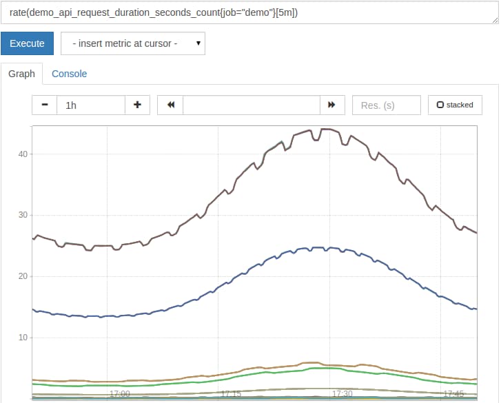
rate() is smart and automatically adjusts for counter resets by assuming that any decrease in a counter value is a reset.
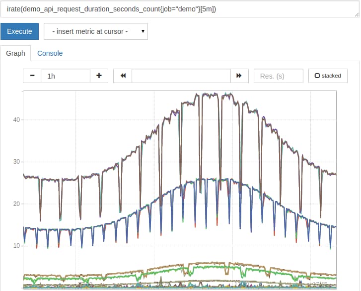
A variant of rate() is irate(). While rate() averages the rate over all samples in the given time window (five minutes in this case), irate() only ever looks back two samples into the past. It still requires you to specify a time window (like [5m]) to know how far to maximally look back in time for those two samples. irate() will react faster to rate changes and is thus usually recommended for use in graphs. In contrast, rate() will provide smoother rates and is recommended for use in alerting expressions (since short rate spikes will be dampened and not wake you up at night).
With irate(), the above graph would look like this, uncovering short intermittent dips in the request rates:
rate() and irate() always calculate a per-second rate. Sometimes you will want to know the total amount by which a counter increased over a window of time but still correct for counter resets. You can achieve this with the increase() function. For example, to calculate the total number of requests handled in the last hour, query for:
increase(demo_api_request_duration_seconds_count{job="demo"}[1h])
Besides counters (which can only increase), there are gauge metrics. Gauges are values that can go up or down over time, like a temperature or free disk space. If we want to calculate changes in gauges over time, we cannot use the rate()/irate()/increase() family of functions. These are all geared towards counters, since they interpret any decrease in the metric value as a counter reset and compensate for it. Instead, we can use the deriv() function, which calculates the per-second derivative of the gauge based on linear regression.
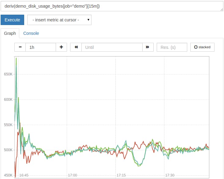
For example, to see how fast a fictional disk usage exported by our demo service is increasing or decreasing (in MiB per second) based on a linear regression of the last 15 minutes, we can query for:
deriv(demo_disk_usage_bytes{job="demo"}[15m])
The result should look like this:
To learn more about calculating deltas and trends in gauges, see also the delta() and predict_linear() functions.
We now know how to calculate per-second rates with different averaging behavior, how counter resets are dealt with in rate calculations, as well as how to compute derivatives for gauges.
Step 6 — Aggregating Over Time Series
In this section, we will learn how to aggregate over individual series.
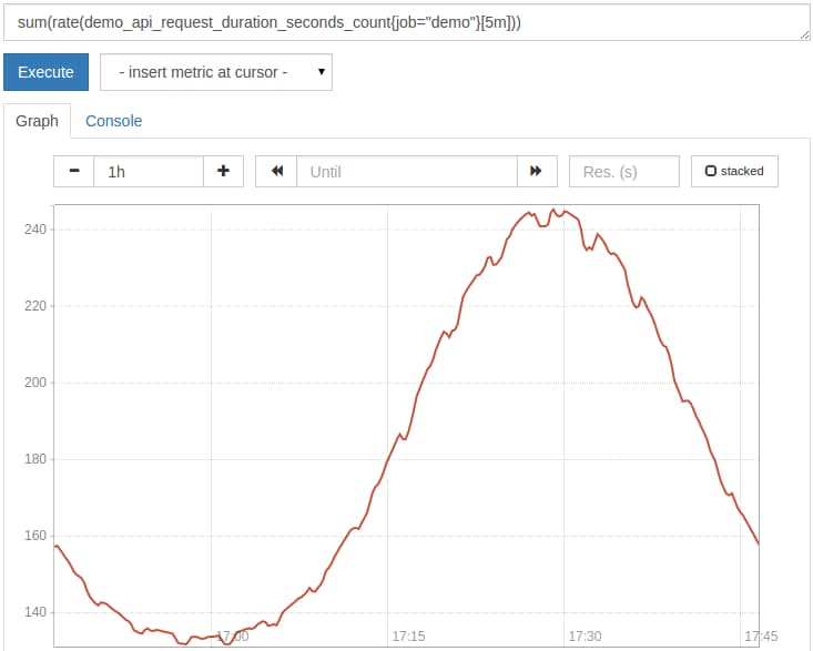
Prometheus collects data with high dimensional detail, which can result in many series for each metric name. However, often you do not care about all dimensions, and you may even have too many series to graph them all at once in a reasonable way. The solution is to aggregate over some of the dimensions and preserve only the ones you care about. For example, the demo service tracks the API HTTP requests by method, path, and status. Prometheus adds further dimensions to this metric when scraping it from the Node Exporter: the instance and job labels that track which process the metrics came from. Now, to see the total request rate over all dimensions, we could use the sum() aggregation operator:
sum(rate(demo_api_request_duration_seconds_count{job="demo"}[5m]))
However, this aggregates over all dimensions and creates a single output series:
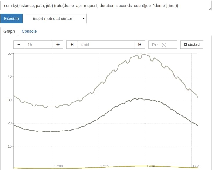
Usually though, you will want to preserve some of the dimensions in the output. For this, sum() and other aggregators support a without(<label names>) clause that specifies the dimensions to aggregate over. There is also an alternative opposite by(<label names>) clause that allows you to specify which label names to preserve. If we wanted to know the total request rate summed over all three service instances and all paths, but split the result up by the method and status code, we could query for:
sum without(method, status) (rate(demo_api_request_duration_seconds_count{job="demo"}[5m]))
This is equivalent to:
sum by(instance, path, job) (rate(demo_api_request_duration_seconds_count{job="demo"}[5m]))
The resulting sum is now grouped by instance, path, and job:
Note: Always calculate the rate(), irate(), or increase() before applying any aggregations. If you applied the aggregation first, it would hide counter resets and these functions would not be able to work properly anymore.
Prometheus supports the following aggregation operators, which each support a by() or without() clause to select which dimensions to preserve:
sum: sums all values within an aggregated group.min: selects the minimum of all values within an aggregated group.max: selects the maximum of all values within an aggregated group.avg: calculates the average (arithmetic mean) of all values within an aggregated group.stddev: calculates the standard deviation of all values within an aggregated group.stdvar: calculates the standard variance of all values within an aggregated group.count: calculates the total number of series within an aggregated group.
You have now learned how to aggregate over a list of series and how to only preserve the dimensions that you care about.
Step 7 — Performing Arithmetic
In this section, we will learn how to do arithmetic in Prometheus.
As the simplest arithmetics example, you can use Prometheus as a numeric calculator. For example, run the following query in the Console view:
(4 + 7) * 3
You will get a single scalar output value of 33:
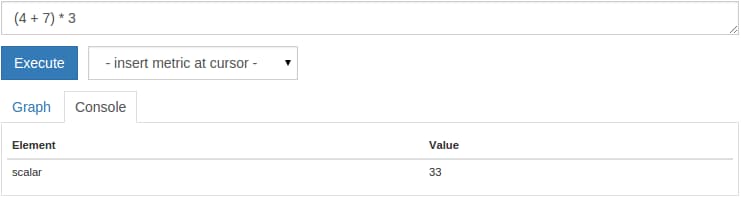
A scalar value is a simple numeric value without any labels. To make this more useful, Prometheus allows you to apply common arithmetic operators (+, -, *, /, %) to entire time series vectors. For example, the following query converts the number of processed bytes by a simulated last batch job run into MiB:
demo_batch_last_run_processed_bytes{job="demo"} / 1024 / 1024
The result will be displayed in MiB:
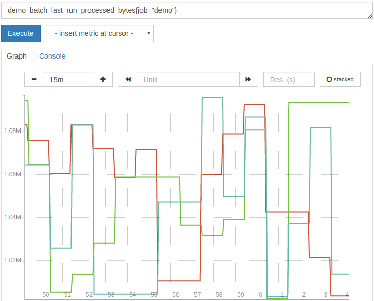
It is common to use simple arithmetic for these types of unit conversions, although good visualization tools (like Grafana) handle conversions for you as well.
A specialty of Prometheus (and where Prometheus really shines!) is binary arithmetic between two sets of time series. When using a binary operator between two sets of series, Prometheus automatically matches elements with identical label sets on the left and right sides of the operation and applies the operator to each matching pair to produce the output series.
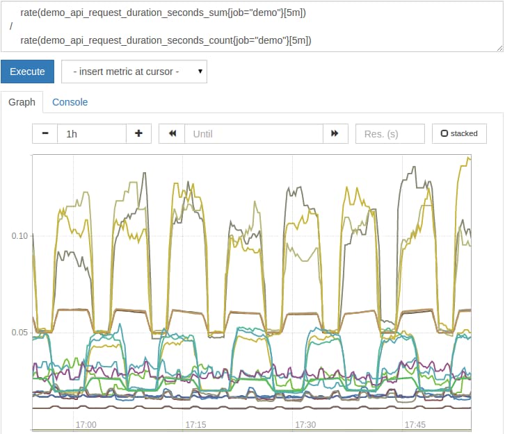
For example, the demo_api_request_duration_seconds_sum metric tells us how many seconds have been spent answering HTTP requests, while demo_api_request_duration_seconds_count tells us how many HTTP requests there were. Both metrics have the same dimensions (method, path, status, instance, job). To calculate the average request latency for each of those dimensions, we can simply query for the ratio of the total time spent in requests divided by the total number of requests.
    rate(demo_api_request_duration_seconds_sum{job="demo"}[5m])
/
    rate(demo_api_request_duration_seconds_count{job="demo"}[5m])
Note that we also wrap a rate() function around each side of the operation to only consider latency for requests that happened in the last 5 minutes. This also adds resiliency against counter resets.
The resulting average request latency graph should look like this:
But what do we do when labels do not match up exactly on both sides? This comes up especially when we have different-sized sets of time series on both sides of the operation, because one side has more dimensions than the other. For example, the demo job exports fictional CPU time spent in various modes (idle, user, system) as a metric demo_cpu_usage_seconds_total with the mode label dimension. It also exports a fictional total number of CPUs as demo_num_cpus (no extra dimensions on this metric). If you tried to divide one by the other to arrive at the average CPU usage in percent for each of the three modes, the query would produce no output:
# BAD!
    # Multiply by 100 to get from a ratio to a percentage
    rate(demo_cpu_usage_seconds_total{job="demo"}[5m]) * 100
/
    demo_num_cpus{job="demo"}
In these one-to-many or many-to-one matchings, we need to tell Prometheus which subset of labels to use for matching, and we also need to specify how to deal with the extra dimensionality. To solve the matching, we add an on(<label names>) clause to the binary operator that specifies the labels to match on. To fan out and group the calculation by the individual values of the extra dimensions on the larger side, we add a group_left(<label names>) or group_right(<label names>) clause that lists the extra dimensions on the left or right side, respectively.
The correct query in this case would be:
    # Multiply by 100 to get from a ratio to a percentage
    rate(demo_cpu_usage_seconds_total{job="demo"}[5m]) * 100
/ on(job, instance) group_left(mode)
    demo_num_cpus{job="demo"}
The result should look like this:
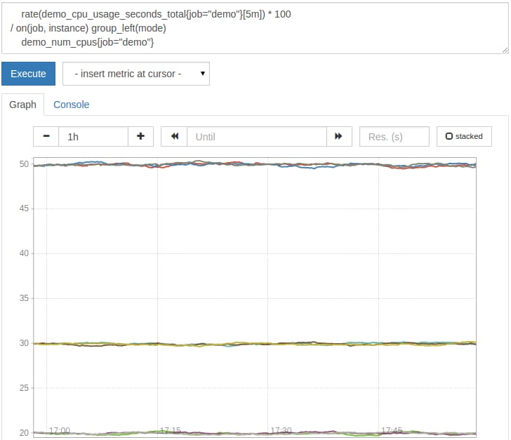
The on(job, instance) tells the operator to only match series from the left and right on their job and instance labels (and thus not on the mode label, which does not exist on the right), while the group_left(mode) clause tells the operator to fan out and display a per-mode CPU usage average. This is a case of many-to-one matching. To do the reverse (one-to-many) matching, use a group_right(<label names>) clause in the same way.
You now know how to use arithmetic between sets of time series, and how to deal with varying dimensions.
Conclusion
In this tutorial, we set up a group of demo service instances and monitored them with Prometheus. We then learned how to apply various query techniques against the collected data to answer questions we care about. You now know how to select and filter series, how to aggregate over dimensions, as well as how to compute rates or derivatives or do arithmetics. You also learned how to approach the construction of queries in general and how to avoid overloading your Prometheus server.
To learn more about Prometheus’s query language, including how to do compute percentiles from histograms, how to deal with timestamp-based metrics, or how to query for service instance health, head on to How To Query Prometheus on Ubuntu 14.04 Part 2.
Thanks for learning with the DigitalOcean Community. Check out our offerings for compute, storage, networking, and managed databases.
Tutorial Series: How To Query Prometheus
We will learn how to query Prometheus 1.3.1. In order to have fitting example data to work with, we will set up three identical demo service instances that export synthetic metrics of various kinds. We will then set up a Prometheus server to scrape and store those metrics. Using the example metrics, we will then learn how to query Prometheus, beginning with simple queries and moving on to more advanced ones.
Browse Series: 2 tutorials
About the author(s)
Co-creator of the Prometheus monitoring system. Infrastructure software developer.
former DO tech editor publishing articles here with the community, then founded the DO product docs team (https://do.co/docs). to all of my authors: you are incredible. working with you was a gift. love is what makes us great.
Still looking for an answer?
This textbox defaults to using Markdown to format your answer.
You can type !ref in this text area to quickly search our full set of tutorials, documentation & marketplace offerings and insert the link!
Is it possible to run scheme as nagios nrpe does? I mean client-server architecture for checks and monitoring system.
I am dealing with a metric K_KA_MP which is a continuous data but it may not come at times to prometheus. So, there are two scenarios two consider -
- query to check that metric was not available in prometheus for the last 5 minutes. Absent function will not be an acceptable solution because there are 4 instances present for the metric and I need to check if metric has stopped coming for one of the instances. Absent will work only when metric is not coming from all 4 instances.
- metric was not available 5 minutes back and it is back now.
Dealing with metric not available in prometheus is proving a nightmare for me because I am unable to track no metric by using any of these aggregate functions. Kindly suggest something for this issue.
Great article. Thank you for taking the time, to put together. Appreciate it sir/madam.
 This work is licensed under a Creative Commons Attribution-NonCommercial- ShareAlike 4.0 International License.
Become a contributor for community
Get paid to write technical tutorials and select a tech-focused charity to receive a matching donation.

DigitalOcean Documentation
Full documentation for every DigitalOcean product.

Resources for startups and AI-native businesses
The Wave has everything you need to know about building a business, from raising funding to marketing your product.
The developer cloud
Scale up as you grow — whether you're running one virtual machine or ten thousand.

Start building today
From GPU-powered inference and Kubernetes to managed databases and storage, get everything you need to build, scale, and deploy intelligent applications.
