By Adrien Payong and Shaoni Mukherjee

Introduction
Suppose you want to understand how different aspects of your personality, such as confidence, communication skills, and body language, contribute to your performance in a job interview. Instead of looking at these factors in isolation, structural equation modeling (SEM) enables the simultaneous analysis of such complex, interconnected relationships. SEM is a multivariate statistical modeling technique that unites factor analysis and regression. This allows researchers to examine both direct and indirect relationships between variables. While traditional regression analysis is typically restricted to observed (measured) variables, SEM can seamlessly incorporate latent variables (theoretical constructs that are not measured directly) and address measurement errors in data. This makes SEM a potent tool for hypothesis testing in psychology, education, marketing, and other social sciences, where many concepts cannot be directly observed.
In this guide, we’ll provide the definition of SEM, discuss the types of models, compare it to regression and factor analysis, and walk you through some practical SEM applications. We’ll also provide a step-by-step SEM example with Python, then show you how to interpret SEM results, discuss the strengths and limitations of SEM, and review some of the latest trends. Whether you’re a researcher trying to test a theoretical model or a data scientist who’s just curious about SEM, this guide will give you a practical, hands-on understanding of structural equation modeling.
Key Takeaways
- SEM integrates factor analysis and regression, allowing for the simultaneous estimation of measurement and structural models.
- Latent variables are unobserved or hypothetical constructs that represent abstract concepts, such as intelligence, satisfaction, or personality traits. These are usually measured indirectly by a set of observed indicators.
- Unlike regression analysis, SEM can accommodate multiple dependent variables, mediators, and indirect effects. It can explicitly account for measurement error in the indicators.
- The model fit to the data is assessed using various indices, like the comparative fit index (CFI), the Tucker-Lewis index (TLI), the root mean square error of approximation (RMSEA), and the standardized root mean square residual (SRMR). The values of these indices indicate how well the proposed model aligns with the observed data.
- SEM is a flexible and widely used technique in many fields, including psychology, education, marketing, and social sciences. It is used to test hypotheses, validate constructs, and explain complex relationships.
Some Key concepts in SEM terminology
Key concepts in SEM terminology include:
- exogenous vs. endogenous variables: An exogenous variable is like an independent variable (there are no arrows pointing at it in the diagram), and an endogenous variable is like a dependent variable, with one or more arrows pointing at it.
- latent vs. observed variables: Latent variables (also known as factors or constructs) are not directly observed but rather are inferred from measured indicators. On the other hand, observed variables are directly measured (e.g., survey items, test scores).
- Path coefficients/factor loadings: Path coefficients are analogous to regression weights, representing the strength of influence between variables. Factor loadings are the connection between latent factors and their observed indicators in the measurement part of the model.
What Is Structural Equation Modeling?
Structural equation modeling refers to a family of statistical methods that allow the construction and testing of multivariable models. It is a highly flexible modeling approach in that the researcher can specify a theoretical model (typically in terms of a set of equations or a path diagram) and then test the extent to which this model fits with the observed data.
At its core, structural equation modeling can be broken down into two components: a measurement model and a structural model. The former is a series of associations between latent variables and observed indicator variables (similar to factor analysis), and the latter is a series of causal (or correlational) associations between latent variables (and possibly observed variables).
A structural model, by contrast, might state that a person’s intelligence (latent) causes some other outcome, such as academic performance (latent or observed). SEM is used to estimate those relationships simultaneously, and also test how well the overall pattern of the model fits the data. Let’s consider the following diagram:
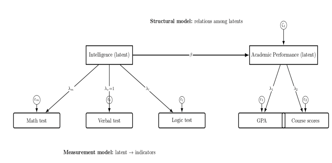
In this diagram, we have a latent variable, Intelligence (measured by the three tests: math, verbal, logic), hypothesized to predict a latent variable, Academic Performance (measured by GPA and course scores). Arrows represent loadings (λ), structural effects (β), and error terms (ε).
The SEM has measurement and structural components. Intelligence is measured by loading onto three test indicators. It drives Academic Performance, which in turn is measured by GPA and course scores. Indicator errors and an endogenous disturbance are represented; one loading is set equal (=1) for identification purposes.
Types of SEM: Measurement vs. Structural Models
SEM is a broad framework that encompasses several types of models. It’s helpful to distinguish between measurement models and structural models, which are often combined in a full SEM:
Measurement Models (Confirmatory Factor Analysis)
Measurement models specify how latent variables are measured by observed indicators. The prototypical example of a measurement model is a confirmatory factor analysis, where you “load” observed variables onto latent factors according to a theoretical model and then check that the data confirm the hypothesized measurement structure.
For example, let’s say you have a theoretical latent construct “Math Ability” which you believe is measured by scores on tests of algebra, geometry, and calculus. In a CFA, you would specify “Math Ability” as a latent factor, with factor paths to those three test score variables.
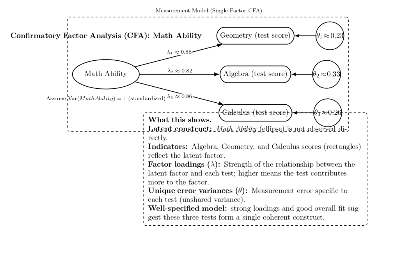
The model will then produce estimates of factor loadings (Like how much each test contributes to the factor) and unique error variances (measurement error unique to each test). A well-specified measurement model will have strong loadings (e.g., high correlation between each test and MathAbility) and a good fit to the data, indicating that the three observed variables indeed form a single construct.
Structural Models (Path Analysis)
These models specify causal (or correlational) relationships among the variables (latent or observed). A path analysis is an SEM with no latent variables (only observed variables, with arrows drawn between them, to represent the presumed cause-and-effect relations or correlations).
Path models can also have mediators (variables that carry an effect from one to another) and reciprocal relationships (with feedback loops), which are not possible in a single regression equation. They can also involve multiple outcomes simultaneously.
In practice, many SEM studies will combine both: a measurement model for each major latent construct in the theory (these are often specified in a CFA first to ensure the measures are good before proceeding further). This will be followed by a structural model linking those latent constructs together ( and perhaps some observed variables). A simple taxonomy of SEM models, then, can be given in terms of what they include:
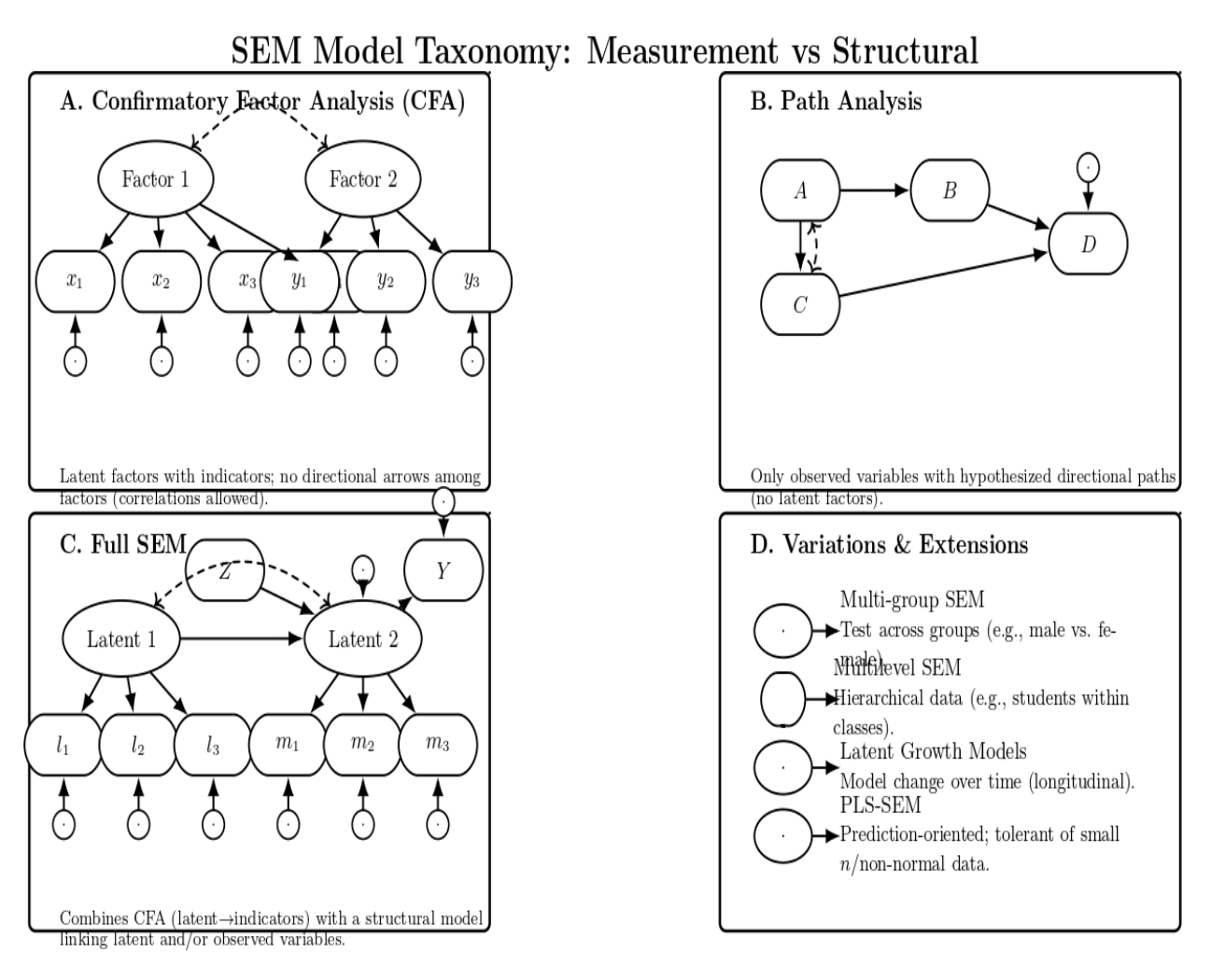
- Confirmatory Factor Analysis (CFA): Only latent variables and their indicators (no directional arrows among the factors, though factors are allowed to correlate).
- Path Analysis: Only observed variables, with directional arrows modeling hypothesized causal paths (no latent factors, so no measurement model needed).
- Full SEM: Latent variables (with their indicators) as well as structural paths among some of the variables (latent or observed). This is the most general case, combining the CFA pieces and regression-like paths in the same overall framework.
- Variations*:* SEM has also been extended in several directions, such as multi-group SEM (testing the same model across different groups of respondents, e.g., does the model hold for males vs females), multilevel SEM (for hierarchical data), and latent growth models (a type of SEM to model change over time using longitudinal data). Another special type of SEM is Partial Least Squares SEM (PLS-SEM), which is a more prediction-oriented approach, more appropriate for smaller samples or non-normal data.
When to Use SEM (SEM vs. Regression vs. Factor Analysis)
Knowing when SEM is the appropriate tool is essential. SEM is best used when research questions involve complex relationships that simpler analyses cannot handle adequately, especially in these scenarios:
- Multiple interrelated dependent variables: When you have multiple outcome variables that might affect each other (e.g., in an education study, the impact of family background on school engagement and the influence of engagement and background on academic achievement), SEM allows you to model all these outcomes and their interrelations simultaneously. Multiple regression would require a set of separate models and could not account for the covariance between outcomes.
- Latent variables and measurement error: If you want to explicitly model latent constructs (e.g., intelligence, socioeconomic status, attitude) that are inferred from several observed measures, SEM is the go-to approach. Unlike ordinary regression that treats each observed measure (which may be noisy) as error-free, SEM can account for measurement error by allowing latent variables to ‘absorb’ the common variance of their associated indicators. This provides more reliable estimates of the relationships between constructs. Regression analysis cannot include latent factors (only observed variables).
- Mediating pathways and complex causal theories: If your theory suggests a network of causal pathways (mediators or moderators). For instance, if you hypothesize that Training → (causes) Motivation → (leads to) Productivity, and also Training → Productivity, you could test these mediation hypotheses with a set of regressions. However, using SEM, you can test the entire chain in a single model. This will provide you with an estimate of direct and indirect effects simultaneously, including a test of overall model fit.
- Model confirmation (confirmatory analysis): If you have a well-specified hypothesis or theoretical model, SEM can provide a plausible confirmatory test. It will tell how well the entire model fits the data, not just individual coefficients. Standard regression could inform you that some predictors are significant, but not whether the hypothesized structure itself is a plausible alternative to other possibilities.
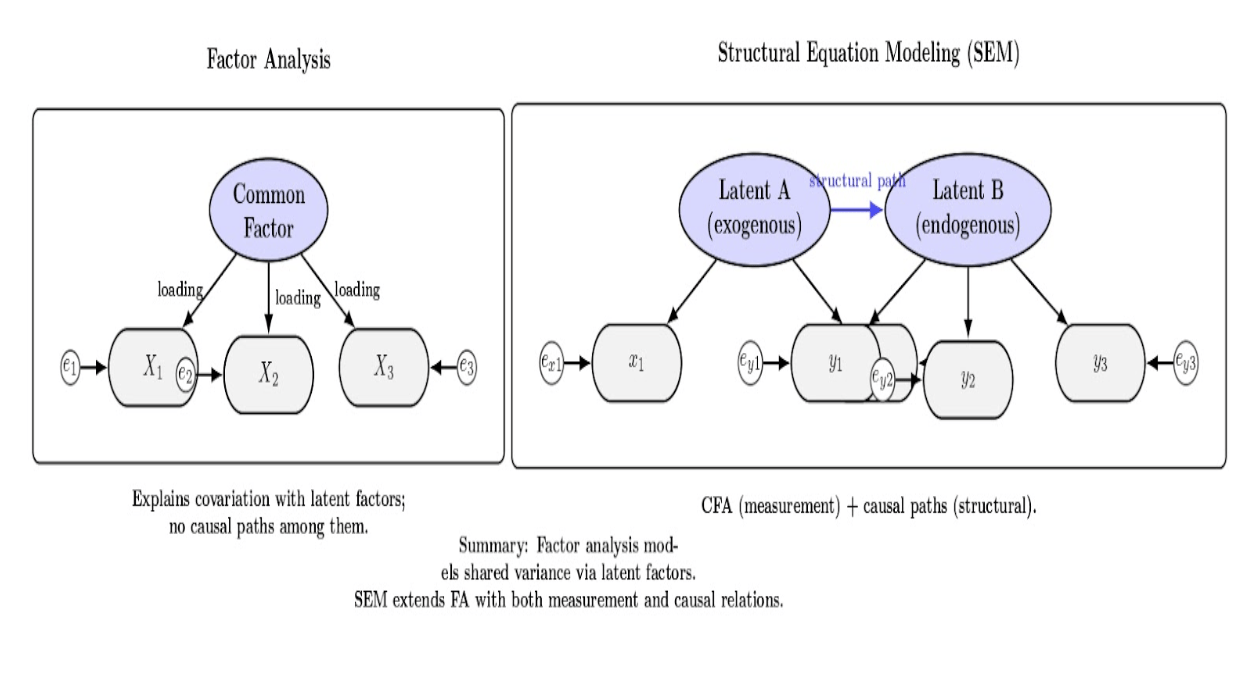
Relation to Factor Analysis
Factor analysis deals with explaining covariation among observed variables through fewer latent factors. SEM is a generalization of this concept: the measurement component of SEM is a confirmatory factor analysis (CFA). The structural component of SEM goes beyond factor analysis by specifying causal relations among latent constructs or between latent and observed variables. Factor analysis does not model causal effects. SEM does.
Applications of SEM in Research
The table below summarizes frequent real-world applications of SEM in various disciplines. It also illustrates how researchers reframe questions from a domain of interest as measurement models (latent constructs) and structural paths (hypothesized effects). Use this table to rapidly map your problem to a SEM template:
- Define the latent constructs.
- Measure the mediators you expect and the outcomes that you care about.
- Then check that your data are suitable for the model (adequate sample size, reliable indicators, and a strong theoretical rationale for the arrows you draw).
| Domain | How SEM Is Applied | Example Scenarios |
|---|---|---|
| Psychology & Social Sciences | Originated and was heavily used in psychology, sociology, and related fields. Model latent constructs like intelligence, personality, attitudes, or well-being. Handle multiple outcomes and confirm whether data support a theorized network of influences. | Educational psychology: latent student traits (motivation, socio-economic status) → academic achievement. Social research: cultural values → behaviors via mediators. PhD dropout study: support, stress, and satisfaction → dropout rates. |
| Marketing & Business Research | Measure customer perceptions and predict outcomes like loyalty or purchase intention. Create indices (customer satisfaction, brand equity) from surveys and test causal links. Accommodate multiple mediators/outcomes and account for measurement error. | Key driver analysis: product attributes → latent factors → satisfaction/likelihood to recommend. Laddering effects: perceptions → attitudes → loyalty. Advertising: ad recall, brand awareness, brand attitude → purchasing (caution: observational data limit causal claims). |
| Education & Sociology | Examine how student background influences performance and institutional outcomes. Combine indicators into latent composites (e.g., socio-economic status). Test complex theoretical frameworks in one integrated model. | Student background (income, parental education) → academic achievement via school quality and motivation. Social capital: neighborhood quality (latent) → life outcomes (employment, health) mediated by education. |
| Healthcare & Epidemiology | Model joint influence of genetic and environmental latent factors on health outcomes. Represent quality of life as a latent construct influenced by multiple domains (mental, physical, and social support). Simultaneously handle measurement error and test mediation; model longitudinal data with latent growth curves. | Genetic + environmental factors → disease risk (with correlations between them). Risk factor → intermediate variables → disease outcome. Track health indicators over time; identify predictors of trajectories. |
| Data Science & Machine Learning | Bring interpretability and causal awareness into predictive analytics. Model latent constructs like “bias” or “fairness perception.” Integrate SEM with machine learning to validate structures and improve explainability. | AI fairness studies: bias/fairness constructs → outcomes or decisions. Confirm clusters or validate recommender system features. User engagement: latent satisfaction & utility → retention. |
Interpreting SEM Results: Fit Indices and Coefficients
After estimating an SEM, two broad types of results are open to interpretation: (1) the goodness-of-fit of the overall model, and (2) the individual parameter estimates (path coefficients, loadings, etc.). Both are essential in SEM reporting.
Model Fit Indices: In contrast to simple regression (where one can look at R² and F-test for the overall model), SEM provides a range of fit indices that need to be considered when interpreting the model’s ability to reproduce the observed data covariance matrix. The table below provides common fit measures and how they can be interpreted.
| Fit Index | What It Assesses | Common Thresholds | Caveats / Notes |
|---|---|---|---|
| Chi-Square Test (χ²) | Difference between the observed covariance matrix and the model-implied covariance matrix. Non-significant χ² suggests the model could plausibly generate the data. | p > 0.05 → good fit. χ²/df ≤ 2–3 is often acceptable | Highly sensitive to sample size (large N can make a trivial misfit “significant”). Rarely used alone; inspect with other indices. |
| CFI (Comparative Fit Index) | Compares the specified model to a baseline independence model (no correlations among variables). Ranges 0–1; closer to 1 is better. | CFI ≥ 0.95 → good fit. CFI ≥ 0.90 → acceptable (in some cases) | Less sensitive to sample size than χ²; still considered alongside RMSEA/SRMR. |
| RMSEA (Root Mean Square Error of Approximation) | Approximate error per degree of freedom; rewards parsimony. Often reported with a 90% CI and p-close. | ≤ 0.05 → close fit. 0.05–0.08 → reasonable fit > 0.10 → poor fit | Prefer RMSEA with confidence interval; smaller values indicate better approximate fit. |
| TLI (Tucker–Lewis Index / NNFI) | Incremental fit index, like CFI, but penalizes model complexity more strongly. | TLI > 0.95 → desired | Can exceed 1 or dip below 0 in rare cases; interpret with other indices. |
| SRMR (Standardized Root Mean Residual) | Average standardized difference between observed and model-implied correlations. | SRMR < 0.08 → good fit | Directly interpretable in correlation units; complements RMSEA/CFI. |
| AIC / BIC (Information Criteria) | Penalized fit measures are used to compare competing models (especially non-nested). | Lower AIC/BIC → preferred model (better fit with parsimony) | Not absolute fit indices; only meaningful for comparison across candidate models. |
Parameter Estimates: Once the model fit is acceptable, you can interpret the path coefficients, factor loadings, and variances:
| Element | What It Captures | How to Interpret (Thresholds & Stats) | Red Flags / Actions |
|---|---|---|---|
| Factor Loadings | Strength with which each observed indicator reflects its latent factor; often standardized. | Significant (p < 0.05) and reasonably large. Rule of thumb: standardized loading ≥ 0.50 is desirable. One loading may be fixed to 1.0 to set the factor’s scale. | Weak/non-significant loading → item may be a poor indicator. Consider revising/removing the indicator or reviewing its measurement quality. |
| Regression Paths | Direction and strength of relationships among variables in the structural model (with SEs and p-values). | Interpret the coefficients controlling for other variables in the model. Report path estimates, SE, p-values, and R² for endogenous variables. | Non-significant hypothesized paths → re-examine theory/power. Very small standardized effects (e.g., 0.10) may be statistically significant but not practically meaningful. |
| Covariances / Correlations | Associations between variables or error terms (two-headed arrows), often used for repeated measures or shared method effects. | Positive, significant covariances are expected for matched indicators over time. Use sparingly and with theoretical justification. | Unexpectedly high residual correlations → possible omitted factor or method effect. Consider adding a theoretically justified latent factor or revising the measurement. |
Structural Equation Modeling in Marketing with Python
We will build an end-to-end SEM pipeline that:
- Simulates a realistic marketing survey with five constructs:
- SQ: Service Quality
- PF: Price Fairness
- CS: Customer Satisfaction
- BL: Brand Loyalty
- PI: Purchase Intention
- Specifies a reflective measurement model and a theory-driven structural model.
- Fits the model with semopy, and inspects standardized estimates and global fit indices (CFI, TLI, RMSEA, SRMR).
- Draw a path diagram.
Install & imports
pip install semopy graphviz
import numpy as np
import pandas as pd
import semopy
from semopy import Model, calc_stats, semplot, report
- semopy fits and inspects SEMs.
- graphviz (system + python package) is needed for diagrams via semplot.
- numpy/pandas handle simulation and data frames.
Simulate latent drivers
# 1) Simulate a marketing survey (replace with your data later)
# ---------------------------
rng = np.random.default_rng(42)
n = 800

# Exogenous latents: SQ & PF with correlation ~ .30
cov_exo = np.array([[1.0, 0.30],
                    [0.30, 1.0]])
SQ, PF = rng.multivariate_normal(mean=[0, 0], cov=cov_exo, size=n).T
The code above:
- Sets a reproducible random number generator and sample size.
- Simulates two exogenous latent variables—Service Quality (SQ) and Price Fairness (PF)—with a correlation ≈ 0.30. In a real-life example, Customers who perceive the service quality to be high are likely to also perceive prices as fair (but not perfectly so).
Simulate downstream latent outcomes via a structural model.
Let’s consider the following code:
# Structural latents
# CS = 0.6*SQ + 0.4*PF + e
e_cs = rng.normal(0, 0.6, n)
CS = 0.6*SQ + 0.4*PF + e_cs

# BL = 0.7*CS + 0.2*SQ + e
e_bl = rng.normal(0, 0.6, n)
BL = 0.7*CS + 0.2*SQ + e_bl

# PI = 0.8*BL + 0.3*CS + e
e_pi = rng.normal(0, 0.6, n)
PI = 0.8*BL + 0.3*CS + e_pi
The structural latents encode a set of variables where CS is expressed as a combination of SQ and PF with an added random noise component. BL is modeled as a function of CS and SQ with additional noise. PI is dependent on BL and CS with some noise. Each of these variables is a linear combination of other variables in the model with some additive normally distributed error. The structural latents represent a linear, causal chain of variables, beginning with SQ and PF, continuing through CS and BL, and ending in PI.
Turn latents into observed survey items (measurement model)
def make_indicators(latent, loads):
    # Simple reflective indicators with Gaussian noise; approx Likert-ish spread
    cols = {}
    for i, lam in enumerate(loads, start=1):
        cols[i] = lam*latent + rng.normal(0, 1 - lam**2, size=len(latent))
    return cols

# Measurement items (factor loadings ~ .6-.9)
SQ_items = make_indicators(SQ, [0.85, 0.80, 0.75, 0.70])
PF_items = make_indicators(PF, [0.80, 0.70, 0.65])
CS_items = make_indicators(CS, [0.85, 0.75, 0.70])
BL_items = make_indicators(BL, [0.80, 0.75, 0.70])
PI_items = make_indicators(PI, [0.85, 0.75, 0.70])
This code simulates observed measurement items as reflective indicators of latent variables. Loadings (or “strengths”) are applied to each latent variable, and Gaussian noise is added to obtain indicators with variability that is proportional to the loadings. The indicators are survey-like in nature (e.g., Likert scales), and the measurement data in this example could be described as realistic simulated data for SQ, PF, CS, BL, and PI.
Assemble the dataset
df = pd.DataFrame({
    # Service Quality
    "SQ1": SQ_items[1], "SQ2": SQ_items[2], "SQ3": SQ_items[3], "SQ4": SQ_items[4],
    # Price Fairness
    "PF1": PF_items[1], "PF2": PF_items[2], "PF3": PF_items[3],
    # Customer Satisfaction
    "CS1": CS_items[1], "CS2": CS_items[2], "CS3": CS_items[3],
    # Brand Loyalty
    "BL1": BL_items[1], "BL2": BL_items[2], "BL3": BL_items[3],
    # Purchase Intention
    "PI1": PI_items[1], "PI2": PI_items[2], "PI3": PI_items[3],
})
This code block places all the generated measurement items into a pandas dataframe, with each column representing a latent construct (SQ, PF, CS, BL, PI) and indicator number.
Declare the SEM (lavaan-style syntax used by semopy)
# 2) Specify SEM in semopy syntax
# ---------------------------
model_desc = """
# Measurement
SQ =~ SQ1 + SQ2 + SQ3 + SQ4
PF =~ PF1 + PF2 + PF3
CS =~ CS1 + CS2 + CS3
BL =~ BL1 + BL2 + BL3
PI =~ PI1 + PI2 + PI3

# Structural
CS ~ SQ + PF
BL ~ CS + SQ
PI ~ BL + CS

# Exogenous correlation
SQ ~~ PF
"""
What it defines:
- =~ provides factor loadings (how items reflect a latent).
- ~ specifies regressions among latents (the structural model).
- ~~ sets a covariance between exogenous latents SQ and PF.
In the code above, the semopy model defines a structural equation model with two components, measurement and structural. The measurement component states that the latent variables SQ, PF, CS, BL, and PI are reflected by their observed indicators. It models direct causal relationships, stating that CS depends on SQ and PF, BL depends on CS and SQ, and PI depends on BL and CS. It also allows SQ and PF to be correlated (exogenous latent variables can be correlated).
Fit the model
# 3) Fit the model
# ---------------------------
model = Model(model_desc)
result = model.fit(df)  # ML by default
print("Converged:", result.success)
print(result)
Output
Converged: True
Name of objective: MLW
Optimization method: SLSQP
Optimization successful.
Optimization terminated successfully
Objective value: 0.111
Number of iterations: 51
Params: 0.937 0.865 0.806 0.849 0.817 0.924 0.794 0.963 0.852 0.891 0.812 0.589 0.426 0.655 0.184 0.821 0.344 0.227 0.812 0.246 0.120 0.200 0.276 0.252 0.087 0.200 0.258 0.596 0.107 0.244 0.385 0.240 0.072 0.182 0.272 0.072 0.128 0.211 0.257
This code fits the defined SEM model to the data in the DataFrame df using semopy’s default Maximum Likelihood Estimation. It then prints whether the optimization has converged and the fitting results, which include parameter estimates and fit statistics.
Inspect parameters (including standardized estimates)
# ---------------------------
# 4) Parameter table (with standardized estimates)
# ---------------------------
est = model.inspect(std_est=True)  # returns DataFrame
# Make columns robust to version differences
def pick(colnames, *cands):
    for c in cands:
        if c in colnames:
            return c
    return None

col_est = pick(est.columns, "Estimate", "Estimates")
col_std = pick(est.columns, "Std. Estimate", "Std Estimate")
print(est.head(15))
  lval op rval  Estimate  Est. Std  Std. Err    z-value p-value
0    CS  ~   SQ  0.588536  0.610210  0.025719  22.883658     0.0
1    CS  ~   PF  0.426119  0.378393  0.031308  13.610467     0.0
2    BL  ~   CS  0.655012  0.663484  0.039701  16.498703     0.0
3    BL  ~   SQ  0.183896  0.193134  0.036458   5.044052     0.0
4    PI  ~   BL  0.820934  0.652613  0.050017  16.413209     0.0
5    PI  ~   CS  0.344395  0.277323  0.047545   7.243527     0.0
6   SQ1  ~   SQ  1.000000  0.958348         -          -       -
7   SQ2  ~   SQ  0.936533  0.920794  0.018449  50.762054     0.0
8   SQ3  ~   SQ  0.865156  0.861719  0.021158  40.890559     0.0
9   SQ4  ~   SQ  0.806385  0.820023  0.022516  35.813445     0.0
10  PF1  ~   PF  1.000000  0.920838         -          -       -
11  PF2  ~   PF  0.849447  0.798678  0.033142   25.63032     0.0
12  PF3  ~   PF  0.816924  0.712679  0.036529  22.363594     0.0
13  CS1  ~   CS  1.000000  0.946910         -          -       -
14  CS2  ~   CS  0.923686  0.873781  0.023139  39.919809     0.0
The script above fits the SEM model to the data and checks for convergence. The resulting parameter table with standardized estimates is then created using model.inspect(std_est=True). The helper function pick is defined to account for potential differences in column names(for estimates and standardized estimates) across semopy versions. The first 15 rows of the parameter table are then printed, showing the estimated model parameters and their standard errors. All paths are statistically significant (p < 0.001), confirming the hypothesized structure. Specifically:
Structural paths
- SQ strongly predicts CS (β ≈ 0.61) and contributes to BL (β ≈ 0.19).
- Price Fairness (PF) also predicts CS (β ≈ 0.38).
- CS drives BL (β ≈ 0.66) and also directly affects Purchase Intention (PI, β ≈ 0.28).
- BL is the strongest predictor of PI (β ≈ 0.65 standardized).
Measurement loadings:
All items (e.g., SQ1–SQ4, PF1–PF3, CS1–CS2, etc.) have strong standardized loadings (mostly above 0.70–0.95). This shows that the indicators reliably measure their constructs.
Check global model fit
This line calculates the global fit indices for the fitted SEM model. The calc_stats() function returns a pandas DataFrame containing common goodness-of-fit statistics such as CFI, TLI, RMSEA, and SRMR. The results are printed in a transposed format, which is easier to read and interpret.
# 5) Global fit indices
# ---------------------------
stats = calc_stats(model)  # DataFrame of CFI, TLI, RMSEA, SRMR, etc.
print(stats.T)
Output:
                     Value
DoF               97.000000
DoF Baseline     120.000000
chi2              88.443733
chi2 p-value       0.720763
chi2 Baseline  12178.091635
CFI                1.000710
GFI                0.992737
AGFI               0.991015
NFI                0.992737
TLI                1.000878
RMSEA              0.000000
AIC               77.778891
BIC              260.478748
LogLik             0.110555
As we can see, all values show outstanding results. The chi-square test is non-significant (χ² = 88.44, p = 0.72), which implies a good fit between the model and the data. All fit indices values (CFI (1.00), TLI (1.00), GFI (0.99), and NFI (0.99)) are above the conventional 0.95 threshold, indicating an excellent fit. An RMSEA of 0.00 means a perfect fit. The AIC and BIC values are relatively low, which further supports that this model is efficient compared to its alternatives.
Visualizing SEM Models with Semopy
import os
png_path = "marketing_sem.png"
try:
    semplot(model, png_path, plot_covs=True, plot_exos=True)  # requires graphviz installed
    if os.path.exists(png_path):
        try:
            from IPython.display import Image, display
            display(Image(filename=png_path))
        except Exception:
            print(f"Diagram saved to: {png_path}")
except Exception as e:
    print("Diagram generation failed (Graphviz not found or other issue):", e)
This code plots the SEM model using semopy’s semplot function and saves it as a PNG file. It requires Graphviz to be installed. If successful, it also attempts to display the image inline (Jupyter notebook, etc. ); otherwise, it prints the file location. If the code block fails (for example, due to missing Graphviz), it prints an error message.
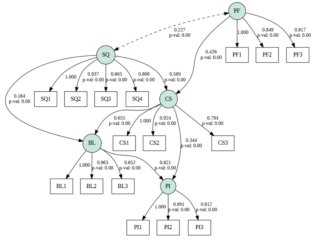
The image displays a path diagram of a structural equation model (SEM) used in marketing research. Latent constructs are represented by circles: service quality (SQ), price fairness (PF), customer satisfaction (CS), brand loyalty (BL), and purchase intention (PI). Rectangular nodes are survey items that are used to measure each construct. The numbers on the arrows are standardized coefficients indicating the magnitude of each relationship. The model shows that all items have high factor loadings on their respective constructs. The structural paths indicate that service quality and price fairness lead to satisfaction, which leads to loyalty, and loyalty is the strongest predictor of purchase intention. The dashed arrow represents a positive correlation between SQ and PF.
Advantages and Limitations of SEM
Like any method, SEM has its pros and cons. Let’s outline them:
Advantages
- Modeling of complex relationships. SEM can model many dependent variables and indirect effects in a single analysis.
- Measurement of latent constructs. Latent variables increase construct validity and decrease measurement error.
- Testing of complex theories. SEM can specify complex networks of relationships and assess direct and indirect effects. Compared with stand-alone regression models, SEM provides more information and richer interpretations.
- Missing data and non‑normality. Modern SEM software uses maximum likelihood with missing data and robust estimators. This makes it appropriate when data are not complete or not normally distributed.
- Visualization. Path diagrams can be useful in communication with non‑statisticians.
- Integration with machine learning. SEM serves as a foundation of interpretable machine learning and causal inference.
Limitations
- Complexity and expertise. SEM models can be conceptually and computationally challenging to develop and understand. Mis‑specification or over‑fitting of the model can lead to erroneous or misleading conclusions.
- Sample size requirements. SEM typically requires large sample sizes. A common rule of thumb is a sample size of at least 200, with 10–20 observations per estimated parameter; smaller samples can result in unstable and biased parameter estimates.
- Linearity and normality assumptions. It assumes linear relationships between variables and multivariate normality of residuals. Violations of these assumptions can lead to biased parameter estimates.
- Model identification. A model must be over‑identified, meaning it has enough information to estimate all of its parameters. Under‑identified models, which lack sufficient information, cannot be estimated.
- Causal ambiguity. SEM can test if the data fit a hypothesized causal model, but it does not establish causality. Multiple competing models may fit the data equally well; strong theoretical justification is required to specify the correct model.
- Software challenges. While many SEM software packages are available (such as AMOS, LISREL, Mplus, EQS, lavaan, and semopy), they vary in terms of features and cost. Some advanced techniques (e.g., Bayesian SEM) may require specialized software.
Emerging Trends: SEM in Machine Learning and Causal Inference
SEM has its roots in 20th-century statistics and social science, but it continues to evolve and find new applications, especially as it intersects with modern computational methods and the growing emphasis on causal inference in data science:
Bayesian and Non‑Parametric SEM
Traditional SEM uses maximum likelihood estimation and assumes multivariate normality. Bayesian SEM uses Bayesian inference to estimate the posterior distributions of the model parameters. This allows the researcher to incorporate prior information on the parameters in the analysis. Bayesian SEM also provides advantages in terms of small samples and non‑normality. The R package blavaan is an extension of lavaan specifically designed for Bayesian models. PyMC and semopy also allow for Bayesian SEM in Python. As promoted by Judea Pearl, Non-parametric SEM is a generalization of SEM that goes beyond linearity to account for non‑linear and non‑Gaussian relationships.
SEM in Machine Learning and Artificial Intelligence
SEM is being combined with machine learning to improve the interpretability of these models and incorporate domain knowledge. For instance, causal neural networks use structural equations to directly constrain the causal structure of deep networks. SEM provides a principled approach to integrating latent variables into neural models and interpreting the hidden layers. Partial least squares SEM and path analysis are also useful complements to unsupervised techniques such as autoencoders. These hybrid techniques are likely to become more prevalent as data sets increase in size and complexity.
Regularization and High‑Dimensional SEM
In high‑dimensional settings (many variables relative to the number of observations), traditional SEM faces challenges related to identification and overfitting. Regularized SEM approaches introduce penalties (e.g., L1, L2) on model parameters to encourage sparsity and improve generalization. The semopy package also supports regularization and random effects models. In addition, other R packages such as regsem, implement penalized SEM. These techniques extend the scalability of SEM to large genetic and brain imaging data sets.
Causal Discovery and Directed Acyclic Graphs
SEM is related to the family of causal graphical models known as directed acyclic graphs. Recent causal discovery algorithms (PC algorithm, Fast Causal Inference) can automatically learn causal structure from data given assumptions about independencies and the absence of latent confounders. The combination of SEM and DAG‑based discovery may enable researchers to build plausible causal models in domains such as genetics, economics, and artificial intelligence.
FAQ SECTION
What is structural equation modeling used for? Structural equation modeling (SEM) is a statistical method that allows you to examine complex relationships between observed (measured) and latent (unobserved) variables. SEM is widely used in various fields, including psychology, education, marketing, and social sciences.
What is the difference between SEM and regression analysis? Regression focuses only on observed variables. It predicts one variable from others. SEM extends regression to include latent variables. It tests an entire system of relationships (measurement model + structural model together).
Which software is best for SEM? There are many software packages available, and the “best” one depends on your needs. Here are some popular ones:
- AMOS (add-on to SPSS): Has a user-friendly, drag-and-drop GUI. Good for beginners.
- LISREL: One of the oldest SEM programs. Very flexible, but with a steep learning curve.
- Mplus: A powerful program that can handle complex models (e.g., multilevel, mixture, longitudinal).
- R (packages lavaan, semopy): Free and open-source, R is one of the most popular options for SEM. Very flexible and can easily be integrated with data science workflows.
- Stata and SAS: They have robust SEM packages and can be used for applied research.
What are common SEM fit indices? The following are some common SEM fit indices to determine how well your model fit to the data:
- Chi-square (χ²): Tests the hypothesis that the model fits the data exactly. It is very sensitive to sample size.
- CFI (Comparative Fit Index): Values greater than 0.90 are considered acceptable, while those greater than 0.95 are considered good.
- TLI (Tucker-Lewis Index): Identical thresholds to the CFI.
- RMSEA (Root Mean Square Error of Approximation): Values less than 0.08 are acceptable, while values less than 0.05 indicate good fit.
- SRMR (Standardized Root Mean Square Residual): Values less than 0.08 are considered good.
Conclusion
Structural equation modeling is a statistical methodology and a way of thinking about complex systems of interrelated constructs or variables. SEM can be applied to diverse fields like social sciences, psychology, marketing, education, economics, and more. Whether you are exploring the effect of personality traits on job performance, analyzing customer satisfaction in marketing research, or testing psychological theories, SEM provides you with a framework to model latent constructs, account for measurement error, and estimate multiple relationships simultaneously.
SEM’s greatest advantage is its ability to operationalize theory. You can take a conceptual model in your mind, translate it into a path diagram, and then test it to see how well it fits reality. The combination of measurement and structural models makes SEM particularly useful in fields where human behavior, perception, or attitude is of interest.
SEM is also rapidly developing and integrating with other areas such as machine learning, causal inference, and big data. Bayesian SEM, regularization for high-dimensional data, and causal discovery are some of the exciting developments that are making SEM more robust, scalable, and flexible. If you are a researcher, analyst, or data scientist who is interested in SEM, or if you want to learn more about it, you have a lot to gain from keeping up with the latest trends and innovations in SEM.
If you’d like to read some other posts that complement SEM and will help you master various data science domains, check out:
References and Resources
- Structural Equation Modeling: Unraveling Complex Relationships in Data
- An Overview Of Structural Equation Modeling (SEM) For Marketing Researchers
- Introduce structural equation modelling to machine learning problems for building an explainable and persuasive model
- Elevating theoretical insight and predictive accuracy in business research: Combining PLS-SEM and selected machine learning algorithms
- The Effect of Perceived Price Fairness, Product Quality, and Service Quality on Customer Loyalty with Customer Satisfaction Mediation on Shopee Consumers
Thanks for learning with the DigitalOcean Community. Check out our offerings for compute, storage, networking, and managed databases.
About the author(s)
I am a skilled AI consultant and technical writer with over four years of experience. I have a master’s degree in AI and have written innovative articles that provide developers and researchers with actionable insights. As a thought leader, I specialize in simplifying complex AI concepts through practical content, positioning myself as a trusted voice in the tech community.
With a strong background in data science and over six years of experience, I am passionate about creating in-depth content on technologies. Currently focused on AI, machine learning, and GPU computing, working on topics ranging from deep learning frameworks to optimizing GPU-based workloads.
Still looking for an answer?
This textbox defaults to using Markdown to format your answer.
You can type !ref in this text area to quickly search our full set of tutorials, documentation & marketplace offerings and insert the link!
 This work is licensed under a Creative Commons Attribution-NonCommercial- ShareAlike 4.0 International License.
Become a contributor for community
Get paid to write technical tutorials and select a tech-focused charity to receive a matching donation.

DigitalOcean Documentation
Full documentation for every DigitalOcean product.

Resources for startups and AI-native businesses
The Wave has everything you need to know about building a business, from raising funding to marketing your product.
The developer cloud
Scale up as you grow — whether you're running one virtual machine or ten thousand.

Start building today
From GPU-powered inference and Kubernetes to managed databases and storage, get everything you need to build, scale, and deploy intelligent applications.
