A Guide to Distilled Stable Diffusion: Implemented with Gradio

SD models are one of the most famous open-source models in general, though most importantly for their capabilities in text-to-image generation. SD has shown exceptional capabilities and has been a backbone in several text-to-image generation applications. SD models are latent diffusion models; the diffusion operations in these models are carried out in a semantically compressed space. Within an SD model, a U-Net performs an iterative sampling to gradually remove noise from a randomly generated latent code. This process is supported by both a text encoder and an image decoder, working collaboratively to generate images that align with provided text descriptions or the prompts. However, this process becomes computationally expensive and often hinders its usage. To tackle the problem, numerous approaches have been introduced.

The study of diffusion models unlocked the potential of compressing the classical architecture to attain a smaller and faster model. The research conducted to achieve a distilled version of SD reduces the sampling steps and applies network quantization without changing the original architectures. This process has shown greater efficiency. This distilled version model demonstrates the efficacy, even with resource constraints.

With just 13 A100 days and a small dataset, this compact model proved to be capable of effectively mimicking the original Stable Diffusion Models (SDMs). Given the cost associated with training SDMs from the ground zero, exceeding 6,000 A100 days and involving 2,000 million pairs, the research shows that network compression emerges as a notably cost-effective approach when constructing compact and versatile diffusion models.

In this tutorial, we will explore the distilled version of Stable Diffusion (SD) through an in-depth guide. This tutorial also includes using Gradio to bring the model to life. Our journey begins with building comprehension of the knowledge distilled version of stable diffusion and its significance.

Furthermore, we will try to break down the model architecture as explained in the associated research paper.

Source

• Distilled Stable Diffusion compresses and optimizes diffusion models for faster performance with minimal accuracy loss.
• It enables real-time or near-real-time image generation on limited GPU resources.
• Gradio integration makes it simple to build and share interactive demos.
• Distillation reduces compute and memory requirements, making it accessible for wider adoption.
• Use cases include art generation, product visualization, prototyping, and creative applications.

• Basic Knowledge of Machine Learning: Understanding of neural networks, especially diffusion models.
• Familiarity with concepts like latent space and image generation.
• Hardware Requirements: A machine with a GPU (NVIDIA CUDA-enabled) for faster inference (e.g., A100, H100, or at least an RTX 20xx/30xx series GPU).
• Environment Setup: Access to Jupyter Notebook or any IDE (e.g., VS Code, PyCharm).
• Basic familiarity with virtual environments (e.g., venv, conda) to avoid conflicts.
• Pre-trained Model Checkpoints: Access to the distilled SD model checkpoints from platforms like Hugging Face Model Hub.

Stable Diffusion belongs to deep learning models called diffusion models. These large text-to-image (T2I) diffusion models work by removing noise from noisy, randomized data. SD models are usually trained on billions of image datasets and are trained to generate new data from what they have learned during the model training.

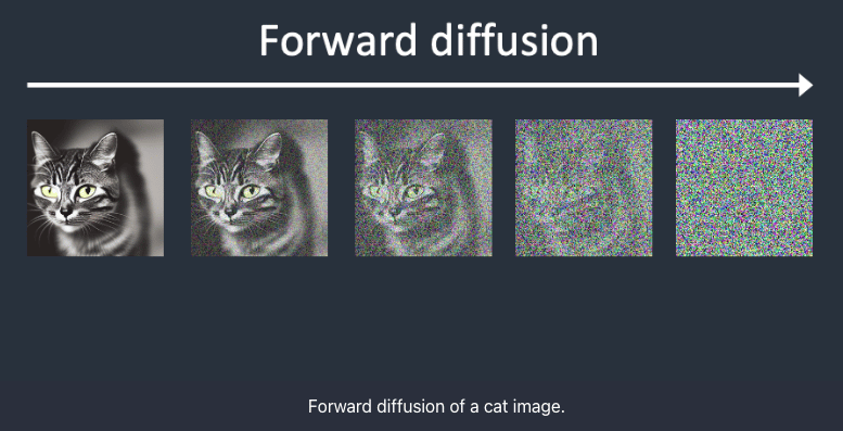
The concept of diffusion begins by adding random noise to an image, let us assume the image to be a cat image. Gradually, by adding noise to the image the image turns to a extremely blurry image which cannot be recognized further. This is called Forward Diffusion.

Source

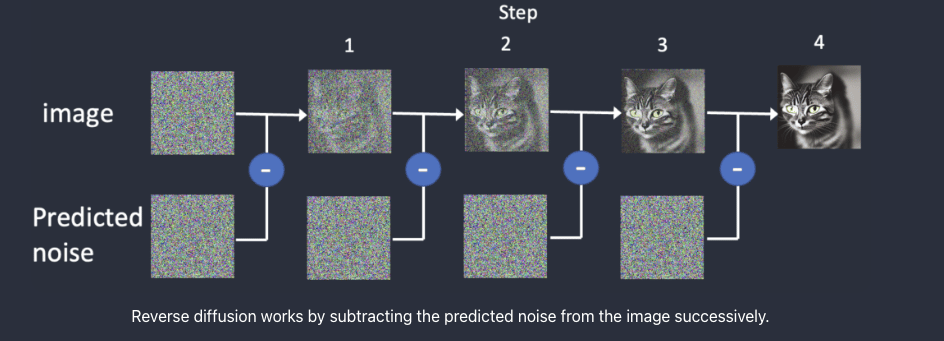
Next, comes the most important part, the Reverse Diffusion. Here, the original image is restored back by removing the noise iteratively. In order to perform Reverse Diffusion, it’s essential to understand the amount of noise introduced to an image. This involves training a deep neural network model to predict the added noise, which is referred to as the noise predictor in Stable Diffusion. The noise predictor takes the form of a U-Net model.

The initial step involves creating a random image and using a noise predictor to predict the noise within that image. Subsequently, we subtract this estimated noise from the original image, and this process is iteratively repeated. After a few iterations, the outcome is an image that represents either a cat or a dog.

Source

However, this process is not an efficient process, and to speed up the process Latent Diffusion Model is introduced. Stable Diffusion functions as a latent diffusion model. Rather than working within the high-dimensional image space, it initially compresses the image into a latent space. This latent space is 48 times smaller, leading to the advantage of processing significantly fewer numbers. This is the reason for its notably faster performance. Stable Diffusion uses a technique called the Variational Autoencoder or VAE neural network. This VAE has two parts: an encoder and a decoder. The encoder compresses the image into a lower-dimensional image, and the decoder restores the image.

During training, instead of generating noisy images, the model generates a tensor in the latent space. Instead of introducing noise directly to an image, Stable Diffusion disrupts the image in the latent space with latent noise. This approach is chosen for its efficiency, as operating in the smaller latent space results in a considerably faster process.

However, here we are talking about images now, the question is from where does the text-to-image come?

In SDMs, a text prompt is passed to a tokenizer to convert it to tokens or numbers. Tokens are numerical values representing the words, and the computer uses them to understand them. Each of these tokens is then converted into a 768-value vector called embedding. Next, the text transformer processes these embeddings. In the end, the output from the transformers is fed to the Noise Predictor U-Net.

[]

Source

The SD model initiates a random tensor in latent space; this random tensor can be controlled by the seed of the random number generator. This noise is the image in the latent space. The Noise predictor takes in this latent noisy image and the prompt and predicts the noise in latent space (4x64x64 tensor).

Furthermore, this latent noise is subtracted from the latent image to generate the new latent image. These steps are iterative, which can be adjusted by the sampling steps. Next, the decoder VAE converts the latent image to pixel space, generating the image aligned with the prompt.

Overall, the latent diffusion model combines elements of probability, generative modeling, and diffusion processes to create a framework for generating complex and realistic data from a latent space.

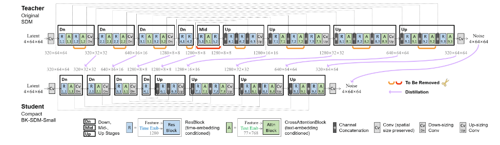
Using Stable Diffusion can be computationally expensive as it involves denoising latents iteratively to generate an image. To reduce the model complexities, the Distilled Stable Diffusion model from Nota AI is introduced. This distilled version streamlines the UNet by removing certain residual and attention blocks of SDM, resulting in a 51% reduction in model size and a 43% improvement in latency on CPU/GPU. This work has been able to achieve greater results and yet has been trained on budget.

As highlighted in the paper “BK-SDM: A Lightweight, Fast, and Cheap Version of Stable Diffusion”, knowledge-distilled SDMs simplify the U-Net, which is the most computationally demanding component of the system. In this setup, the U-Net—conditioned on both text and time-step information—performs iterative denoising to generate latent representations. By reducing the per-step computations within the U-Net, the model achieves greater efficiency. The compressed architecture derived from SDM-v1 is illustrated in the figure below.

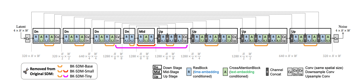
Image from original Research Paper

Let’s begin by installing the required libraries. In addition to the DSD libraries, we will also install Gradio.

!pip install --quiet git+https://github.com/huggingface/diffusers.git@d420d71398d9c5a8d9a5f95ba2bdb6fe3d8ae31f
!pip install --quiet ipython-autotime
!pip install --quiet transformers==4.34.1 accelerate==0.24.0 safetensors==0.4.0
!pip install --quiet ipyplot
!pip install gradio
%load_ext autotime

Next, we will build a pipeline and generate the first image and save the generated image.

# Import the necessary libraries

from diffusers import StableDiffusionXLPipeline
import torch
import ipyplot
import gradio as gr

pipe = StableDiffusionXLPipeline.from_pretrained("segmind/SSD-1B", torch_dtype=torch.float16, use_safetensors=True, variant="fp16")
pipe.to("cuda")


prompt = "an orange cat staring off with pretty eyes, Striking image, 8K, Desktop background, Immensely sharp." 
neg_prompt = "ugly, poorly Rendered face, low resolution, poorly drawn feet, poorly drawn face, out of frame, extra limbs, disfigured, deformed, body out of frame, blurry, bad composition, blurred, watermark, grainy, signature, cut off, mutation"

image = pipe(prompt=prompt, negative_prompt=neg_prompt).images[0]

image.save("test.jpg") 

ipyplot.plot_images([image],img_width=400)

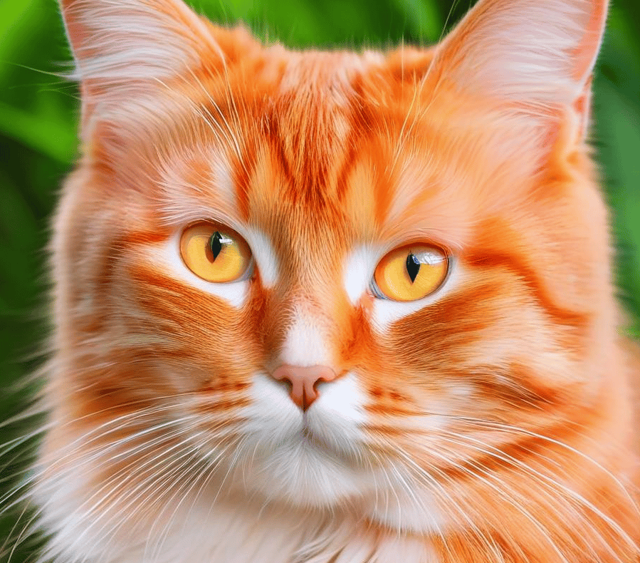
Image Result

The above code imports the ‘StableDiffusionXLPipeline’ class from the ‘diffusers’ module. Post-importing the necessary libraries, we will create an instance of the ‘StableDiffusionXLPipeline’ class named ‘pipe.’ Next, load the pre-trained model named “segmind/SSD-1B” into the pipeline. The model is configured to use 16-bit floating-point precision that we specify in the dtype argument, and safe tensors are enabled. The variant is set to “fp16”. Since we will use 'GPU, we will move the pipeline to a CUDA device for faster computation.

Let us enhance the code further, by adjusting the guidance scale, which impacts the prompts on the image generation. In this case, it is set to 7.5. The parameter ‘num_inference_steps’ is set to 30, this number indicates the steps to be taken during the image generation process.

allimages = pipe(prompt=prompt, negative_prompt=neg_prompt,guidance_scale=7.5,num_inference_steps=30,num_images_per_prompt=2).images

Gradio provides the quickest method to showcase your machine learning model through a user-friendly web interface, enabling accessibility for anyone to use. Let us learn how to build a simple UI using Gradio.

Define a function to generate the images that we will use to build the Gradio interface.

def gen_image(text, neg_prompt):
    return pipe(text,
                negative_prompt=neg_prompt,
                guidance_scale=7.5,
                num_inference_steps=30).images[0]

Next, the code snippet utilizes the Gradio library to create a simple web interface for generating AI-generated images using a function called gen_image.

txt = gr.Textbox(label="prompt")
txt_2 = gr.Textbox(label="neg_prompt")

Two textboxes (txt and txt_2) are defined using the gr.Textbox class. These textboxes serve as input fields where users can enter text data. They are used for entering the prompt and the negative prompt.

#Gradio Interface Configuration
demo = gr.Interface(fn=gen_image, inputs=[txt, txt_2], outputs="image", title="Generate A.I. image using Distill Stable Diffusion😁")
demo.launch(share=True)

• First, specify the function gen_image as the function to be executed when the interface receives input.
• Defines the input components for the interface, which are the two textboxes for the prompt and negative prompt (txt and txt_2).
• outputs="image": generate the image output and set the title of the interface title="Generate A.I. image using Distill Stable Diffusion😁"
• The launch method is called to start the Gradio interface. The share=True parameter indicates that the interface should be made shareable, allowing others to access and use it.

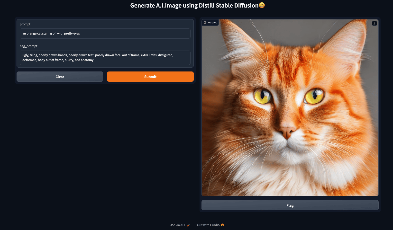
In summary, this code sets up a Gradio interface with two textboxes for user input, connects it to a function (gen_image) for processing, specifies that the output is an image, and launches the interface for sharing. We can input prompts and negative prompts in the textboxes to generate AI-generated images through the provided function.

The SSD-1B model

Recently, Segmind launched the open source foundation model, SSD-1B, and has claimed to be the fastest diffusion text-to-image model. Developed as a part of the distillation series, SSD-1B shows a 50% reduction in size and a 60% increase in speed when compared with the SDXL 1.0 model. Despite these improvements, there is only a marginal compromise in image quality compared to SDXL 1.0. Additionally, the SSD-1B model has obtained commercial licensing, providing businesses and developers with the opportunity to incorporate this cutting-edge technology into their offerings.

This model is the distilled version of the SDXL, and it has proven to generate images of superior quality faster while being affordable.

The NotaAI/bk-sdm-small

Another distilled version of SD from Nota AI is very common for T2I generations. The Block-removed Knowledge-distilled Stable Diffusion Model (BK-SDM) represents a structurally streamlined version of SDM, designed for efficient general-purpose text-to-image synthesis. Its architecture involves (i) eliminating multiple residual and attention blocks from the U-Net of Stable Diffusion v1.4 and (ii) pretraining through distillation using only 0.22M LAION pairs, which is less than 0.1% of the complete training set. Despite the use of significantly restricted resources in training, this compact model demonstrates the ability to mimic the original SDM through the effective transfer of knowledge.

Is the Distilled Version really fast?

Now, the question arises: are these distilled versions of SD really fast, and there is only one way to find out.

In this evaluation, we will assess four models belonging to the diffusion family. We will use segmind/SSD-1B, stabilityai/stable-diffusion-xl-base-1.0, nota-ai/bk-sdm-small, and CompVis/stable-diffusion-v1-4 for our evaluation purposes. Please feel free to click on the link for a detailed comparative analysis of SSD-1B and SDXL.

Let us load all the models and compare them:

import torch
import time
import ipyplot

from diffusers import StableDiffusionPipeline, StableDiffusionXLPipeline, DiffusionPipeline

In the code snippet below, we will use four different pre-trained models from the Stable Diffusion family to create a pipeline for text-to-image synthesis.

#text-to-image synthesis pipeline using the "bk-sdm-small" model from nota-ai
distilled = StableDiffusionPipeline.from_pretrained(
    "nota-ai/bk-sdm-small", torch_dtype=torch.float16, use_safetensors=True,
).to("cuda")

#text-to-image synthesis pipeline using the "stable-diffusion-v1-4" model from CompVis
original = StableDiffusionPipeline.from_pretrained(
    "CompVis/stable-diffusion-v1-4", torch_dtype=torch.float16, use_safetensors=True,
).to("cuda")

#text-to-image synthesis pipeline using the original "stable-diffusion-xl-base-1.0" model from stabilityai
SDXL_Original = DiffusionPipeline.from_pretrained(
    "stabilityai/stable-diffusion-xl-base-1.0", torch_dtype=torch.float16, 
    use_safetensors=True, variant="fp16"
).to("cuda")

#text-to-image synthesis pipeline using the original "SSD-1B" model from segmind
ssd_1b = StableDiffusionXLPipeline.from_pretrained(
    "segmind/SSD-1B", torch_dtype=torch.float16, use_safetensors=True, 
    variant="fp16"
).to("cuda")

Once the model is loaded and the pipelines are created, we will use these models to generate a few images and check the inference time for each model. Please note here that all the model pipelines should not be included in a single cell; otherwise, one might encounter memory issues.

Model

Inference Time

stabilityai/stable-diffusion-xl-base-1.0

82212.8 ms

segmind/SSD-1B

59382.0 ms

CompVis/stable-diffusion-v1-4

15356.6 ms

nota-ai/bk-sdm-small

10027.1 ms

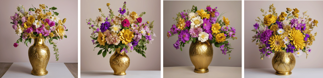
The bk-sdm-small model took the least amount of inference time, additionally the model was able to generate high quality images.

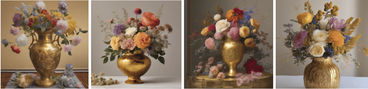
stabilityai/stable-diffusion-xl-base-1.0

segmind/SSD-1B

CompVis/stable-diffusion-v1-4

nota-ai/bk-sdm-small

1. What is Distilled Stable Diffusion?

Distilled Stable Diffusion is a lighter, faster version of the original Stable Diffusion model. Through a process called model distillation, it reduces the size and complexity of the model while keeping its ability to generate high-quality images. This makes it more efficient and easier to run on limited GPU hardware.

2. How does model distillation improve performance?

Model distillation transfers knowledge from a large model (the “teacher”) to a smaller one (the “student”). The student model learns to replicate the teacher’s performance but with fewer parameters. This process improves inference speed, lowers memory usage, and reduces computational costs, making it suitable for real-time applications.

3. Why integrate Distilled Stable Diffusion with Gradio?

Gradio provides a simple, user-friendly interface for deploying machine learning models. With Gradio, users can input text prompts and instantly see generated images, without needing coding expertise. It also makes it easy to share demos via a link or embed them in applications, fostering collaboration and accessibility.

4. What are the advantages of using Distilled Stable Diffusion over the original model?

The main benefits include:

• Faster inference (generates images more quickly). Lower hardware requirements, making it runnable on consumer GPUs or cloud GPUs.
• Cost efficiency for cloud-based deployments.
• Wider accessibility, enabling more people to experiment with generative AI.

5. What are some practical use cases?

Distilled Stable Diffusion can be applied in:

• Creative arts (digital painting, concept art, design prototypes).
• Marketing and advertising (generating visuals for campaigns).
• E-commerce (product visualization).
• Education and research (explaining generative AI concepts with a lightweight model).

6. How can I run Distilled Stable Diffusion if I don’t have a powerful GPU?

You can use cloud GPUs like DigitalOcean Gradient™ AI GPU Droplets, which provide flexible access to high-performance GPUs without upfront investment. This makes it easy to train or deploy distilled models while only paying for what you use.

In this article, we provided a concise overview of the Stable Diffusion model and explored the concept of Distilled Stable Diffusion. Stable Diffusion (SD) emerges as a potent technique for generating new images through straightforward prompts. Additionally, we examined four models within the SD family, highlighting that the bk-sdm-small model demonstrated the shortest inference time. This shows how efficient KD models are compared to the original model.

It is also important to acknowledge that the distilled model has certain limitations. Firstly, it doesn’t attain flawless photorealism, and legible text rendering is beyond its current capabilities. Moreover, when confronted with complex tasks requiring compositional understanding, the model’s performance may drop. Additionally, facial and general human representations might not be generated accurately. It’s crucial to note that the model’s training data primarily consists of English captions, which can result in reduced effectiveness when applied to other languages.

It is important to note that the models used should not be utilized to generate disturbing, distressing, or offensive images. A key advantage of distilling these high-performing models is the significant reduction in computational requirements while maintaining the generation of high-quality images.

• Stable Diffusion
• Inference with SSD 1B — A distilled Stable Diffusion XL model that is 50% smaller and 60% faster
• Announcing SSD-1B: A Leap in Efficient T2I Generation
• Stable Diffusion pipelines
• Distilled Stable Diffusion inference
• nota-ai/bk-sdm-small
• stabilityai/stable-diffusion-xl-base-1.0
• BK-SDM: A Lightweight, Fast, and Cheap Version of Stable Diffusion