Tutorial

Data Augmentation for Bounding Boxes: Rotation and Shearing

Updated on April 7, 2025

Data Augmentation for Bounding Boxes: Rotation and Shearing

Introduction

When training a computer vision or object detection model, the quality and variety of your dataset play a huge role in how well the model performs. However, collecting and labeling large amounts of real-world data is time-consuming and expensive. That’s where data augmentation comes in—by applying transformations like rotation and shearing, we can artificially expand our dataset and make the model more robust.

Imagine you’re training a model to detect cars in images. If all the images show cars from a straight-on angle, the model might struggle when it sees a car from a tilted perspective. Rotation helps the model learn to recognize objects from different angles, while shearing slightly distorts the image to mimic real-world variations, making the model more adaptable.

These augmentation techniques improve the model’s accuracy, reduce overfitting, and make it more reliable in real-world scenarios—without needing extra labeled data. In this article, we’ll explore how to apply rotation and shearing to bounding boxes effectively and why these techniques are essential for building high-performing object detection models.

Prerequisites

Before diving into bounding box augmentation with rotation and shearing, it’s helpful to be familiar with the following:

Basic understanding of image augmentation – Know how image transformations like rotation, flipping, and scaling work.
Bounding boxes – Understand how objects in images are labeled using bounding boxes (typically with coordinates like x_min, y_min, x_max, y_max).
Coordinate geometry – Since transformations involve modifying box positions, a basic grasp of coordinate systems will be useful.
Python and NumPy – You’ll need to write simple code to apply transformations and update bounding box coordinates.

GitHub Repo

You can find all the techniques covered in this article, along with the complete augmentation library, in the GitHub repository: Now, let’s dive in!

Rotation

Rotation is one of the nastiest data augmentations. Soon you will know why.

Affine Transformation: A transformation of an image such that parallel lines in an image remain parallel after the transformation. Scaling, translation, and rotation are all examples of affine transformations.

In computer graphics, we also use a transformation matrix, a convenient tool to carry out affine transformations.

A full discussion of the transformation matrix is beyond the scope of this article. However, you can think of it as a mathematical tool used to manipulate a point’s coordinates. By multiplying a point’s coordinates with the transformation matrix, you obtain the new, transformed position, which is essential in operations like rotation, scaling, and translation in geometry and computer graphics.

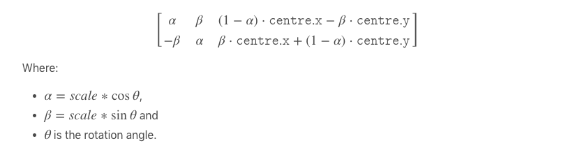
The transformation matrix is a 2 x 3 matrix multiplied by [x y 1], where (x,y) are the coordinates of the point. The idea of having a 1 is to facilitate sharing, and you can read more about it in the link below. Multiplying a 2 x 3 matrix with a 3 x 1 matrix leaves us with a 2 x 1 matrix containing the new point coordinates. The transformation matrix can also be used to get the coordinates of a point after rotation about the center of the image. The transformation matrix for rotating a point by θ, theta looks like.

Thankfully, we won’t have to code it. OpenCV already provides built-in functionality for doing it using its cv2.warpAffine function. So, with the requisite theoretical knowledge behind us, let’s get started.

We start by defining our __init__ function.

def __init__(self, angle = 10):
    self.angle = angle

    if type(self.angle) == tuple:
        assert len(self.angle) == 2, "Invalid range"   
    else:
        self.angle = (-self.angle, self.angle)

Rotating the Image

Now, the first thing we have to do is rotate our image by an angle θ about the center. For this, we need our transformation matrix. We use the OpenCV function getRotationMatrix2D for this.

(h, w) = image.shape[:2]
(cX, cY) = (w // 2, h // 2)
M = cv2.getRotationMatrix2D((cX, cY), angle, 1.0)

Now, we can get the rotated image by using the warpAffine function.

image = cv2.warpAffine(image, M, (w, h))

The third argument to the function is (w,h) because we want to maintain the original resolution. But if you imagine a bit, a rotated image will have different dimensions, and if they exceed the original dimensions, OpenCV will simply cut them. Here is an example.

OpenCV rotation side-effect.

We lose some information here. So, how do we get past that? Thankfully, OpenCV provides us with an argument to the function that helps us determine the dimensions of the final image. If we can change it from (w,h) to a dimension that will just accommodate our rotated image, we are done.

This idea is inspired by Adrian Rosebrock’s post on PyImageSearch, where he explores it in detail.

Now, the question is, how do we find these new dimensions? A little trigonometry can do the job for us. Take a look at the following diagram.

Image source

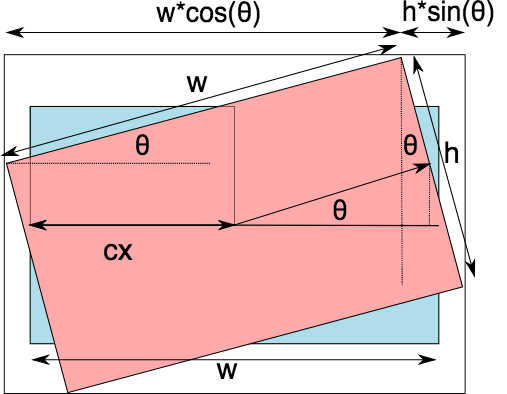
This image illustrates the effect of rotating a rectangular object by an angle θ and how its dimensions change after the transformation. Here’s a breakdown of the key elements in the diagram:

Original and Rotated Rectangles

The blue rectangle represents the original unrotated object with width w and height h.
The red rectangle represents the rotated version of the same object at an angle theta.

Transformation Components

The new bounding box (outermost white rectangle) must enclose the rotated object.
The rotated width and height are extended due to the trigonometric effects of rotation.

Trigonometric Calculations

The transformed width extends due to the horizontal component of the original width and the vertical component of the original height.
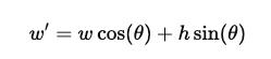
Similarly, the transformed height is computed as

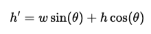
This equation represents the bounding box adjustments in image processing when rotation is applied in image transformation. When an object is rotated, the new bounding box needs to be calculated to ensure it fully contains the transformed shape.

cos = np.abs(M[0, 0])
sin = np.abs(M[0, 1])

# compute the new bounding dimensions of the image
nW = int((h * sin) + (w * cos))
nH = int((h * cos) + (w * sin))

There’s something still missing. One thing is sure: the center of the image does not move since it is the axis of rotation itself. However, since the width and height of the image are now nW and nH, the center must lie at nW/2 and nH/2. To ensure this happens, we must translate the image by nW/2 - cX nH/2 - cH, where cX and cH are the previous centers.

# adjust the rotation matrix to take into account translation
M[0, 2] += (nW / 2) - cX
M[1, 2] += (nH / 2) - cY

To sum this up, we put the code responsible for rotating an image in a function rotate_im and place it in the bbox_util.py

def rotate_im(image, angle):
    """Rotate the image.

    Rotate the image such that the rotated image is enclosed inside the tightest
    rectangle. The area not occupied by the pixels of the original image is colored
    black. 

    Parameters
    ----------

    image : numpy.ndarray
        numpy image

    angle : float
        angle by which the image is to be rotated

    Returns
    -------

    numpy.ndarray
        Rotated Image

    """
    # grab the dimensions of the image and then determine the
    # centre
    (h, w) = image.shape[:2]
    (cX, cY) = (w // 2, h // 2)

    # grab the rotation matrix (applying the negative of the
    # angle to rotate clockwise), then grab the sine and cosine
    # (i.e., the rotation components of the matrix)
    M = cv2.getRotationMatrix2D((cX, cY), angle, 1.0)
    cos = np.abs(M[0, 0])
    sin = np.abs(M[0, 1])

    # compute the new bounding dimensions of the image
    nW = int((h * sin) + (w * cos))
    nH = int((h * cos) + (w * sin))

    # adjust the rotation matrix to take into account translation
    M[0, 2] += (nW / 2) - cX
    M[1, 2] += (nH / 2) - cY

    # perform the actual rotation and return the image
    image = cv2.warpAffine(image, M, (nW, nH))

#    image = cv2.resize(image, (w,h))
    return image

Rotating the Bounding Box

This is the most challenging part of this augmentation. Here, we first need to rotate the bounding box, which gives us a tilted rectangular box. Then, we have to find the tightest rectangle parallel to the sides of the image containing the tilted rectangular box.

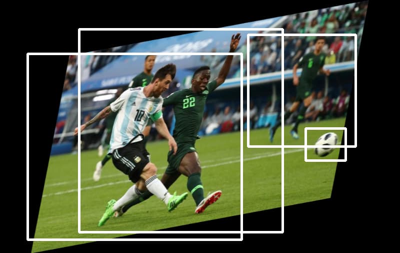
Here is what I mean.

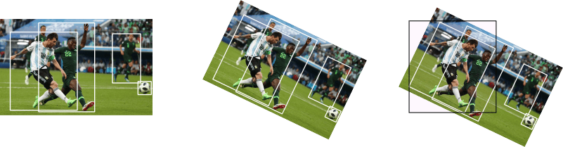Final Bounding Box, shown only for one image.

Now, to get the rotated bounding box, as seen in the middle image, we need all the coordinates for all four corners of the box.

We could actually get the final bounding box using only two corners, but that would take more trigonometry to figure out the dimensions of the final bounding box (on the right in the image above, in black) using only two corners. With four corners of the intermediate box in the middle, it’s much easier to make that computation. It’s only a matter of making the code more complicated.

So, first, we write the function get_corners in the file bbox_utils.py to get all four corners.

def get_corners(bboxes):
    
    """Get corners of bounding boxes

    Parameters
    ----------

    bboxes: numpy.ndarray
        Numpy array containing bounding boxes of shape `N X 4` where N is the 
        number of bounding boxes and the bounding boxes are represented in the
        format `x1 y1 x2 y2`

    returns
    -------

    numpy.ndarray
        Numpy array of shape `N x 8` containing N bounding boxes each described by their 
        corner co-ordinates `x1 y1 x2 y2 x3 y3 x4 y4`      

    """
    width = (bboxes[:,2] - bboxes[:,0]).reshape(-1,1)
    height = (bboxes[:,3] - bboxes[:,1]).reshape(-1,1)

    x1 = bboxes[:,0].reshape(-1,1)
    y1 = bboxes[:,1].reshape(-1,1)

    x2 = x1 + width
    y2 = y1 

    x3 = x1
    y3 = y1 + height

    x4 = bboxes[:,2].reshape(-1,1)
    y4 = bboxes[:,3].reshape(-1,1)

    corners = np.hstack((x1,y1,x2,y2,x3,y3,x4,y4))

    return corners

After this, each bounding box is described by eight coordinates: x1,y1,x2,y2,x3,y3,x4,y4. We now define the function rotate_box in the file bbox_util.py, which rotates the bounding boxes for us by giving us the transformed points. We use the transformation matrix for this.

def rotate_box(corners,angle,  cx, cy, h, w):
    
    """Rotate the bounding box.


    Parameters
    ----------

    corners : numpy.ndarray
        Numpy array of shape `N x 8` containing N bounding boxes each described by their 
        corner co-ordinates `x1 y1 x2 y2 x3 y3 x4 y4`

    angle : float
        angle by which the image is to be rotated

    cx : int
        x coordinate of the center of image (about which the box will be rotated)

    cy : int
        y coordinate of the center of image (about which the box will be rotated)

    h : int 
        height of the image

    w : int 
        width of the image

    Returns
    -------

    numpy.ndarray
        Numpy array of shape `N x 8` containing N rotated bounding boxes each described by their 
        corner co-ordinates `x1 y1 x2 y2 x3 y3 x4 y4`
    """

    corners = corners.reshape(-1,2)
    corners = np.hstack((corners, np.ones((corners.shape[0],1), dtype = type(corners[0][0]))))

    M = cv2.getRotationMatrix2D((cx, cy), angle, 1.0)


    cos = np.abs(M[0, 0])
    sin = np.abs(M[0, 1])

    nW = int((h * sin) + (w * cos))
    nH = int((h * cos) + (w * sin))
    # adjust the rotation matrix to take into account translation
    M[0, 2] += (nW / 2) - cx
    M[1, 2] += (nH / 2) - cy
    # Prepare the vector to be transformed
    calculated = np.dot(M,corners.T).T

    calculated = calculated.reshape(-1,8)

    return calculated

Now, the final thing is to define a function get_enclosing_box, which gets us the tightest box talked about.

def get_enclosing_box(corners):
    """Get an enclosing box for ratated corners of a bounding box
    
    Parameters
    ----------
    
    corners : numpy.ndarray
        Numpy array of shape `N x 8` containing N bounding boxes each described by their 
        corner co-ordinates `x1 y1 x2 y2 x3 y3 x4 y4`  
    
    Returns 
    -------
    
    numpy.ndarray
        Numpy array containing enclosing bounding boxes of shape `N X 4` where N is the 
        number of bounding boxes and the bounding boxes are represented in the
        format `x1 y1 x2 y2`
        
    """
    x_ = corners[:,[0,2,4,6]]
    y_ = corners[:,[1,3,5,7]]
    
    xmin = np.min(x_,1).reshape(-1,1)
    ymin = np.min(y_,1).reshape(-1,1)
    xmax = np.max(x_,1).reshape(-1,1)
    ymax = np.max(y_,1).reshape(-1,1)
    
    final = np.hstack((xmin, ymin, xmax, ymax,corners[:,8:]))
    
    return final

This again gives us a notation in which four coordinates or two corners determine each bounding box. Using all these helper functions, we finally put together our __call__ function.

def __call__(self, img, bboxes):

    angle = random.uniform(*self.angle)

    w,h = img.shape[1], img.shape[0]
    cx, cy = w//2, h//2

    img = rotate_im(img, angle)

    corners = get_corners(bboxes)

    corners = np.hstack((corners, bboxes[:,4:]))


    corners[:,:8] = rotate_box(corners[:,:8], angle, cx, cy, h, w)

    new_bbox = get_enclosing_box(corners)


    scale_factor_x = img.shape[1] / w

    scale_factor_y = img.shape[0] / h

    img = cv2.resize(img, (w,h))

    new_bbox[:,:4] /= [scale_factor_x, scale_factor_y, scale_factor_x, scale_factor_y] 

    bboxes  = new_bbox

    bboxes = clip_box(bboxes, [0,0,w, h], 0.25)

    return img, bboxes

Notice that at the end of the function, we rescale our image and the bounding boxes so that our final dimensions are w,h, and not nW, nH. This is just to preserve the dimensions of the image. We also clip boxes in case any box may be out of the image after transformation.

Shearing

Shearing is another bounding box transformation that can be performed with the help of the transformation matrix.

The effect that shearing produces is shown below.

In shearing, we turn the rectangular image into a parallelogram image. The transformation matrix used in shearing is.

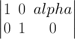
The above is an example of a horizontal shear. In this, the pixel with coordinates x, y is moved to x + alpha*y, y. alpha is the shearing factor. We therefore define our __init__ function as.

class RandomShear(object):
    """Randomly shears an image in horizontal direction   
    
    
    Bounding boxes which have an area of less than 25% in the remaining in the 
    transformed image is dropped. The resolution is maintained, and the remaining
    area if any is filled by black color.
    
    Parameters
    ----------
    shear_factor: float or tuple(float)
        if **float**, the image is sheared horizontally by a factor drawn 
        randomly from a range (-`shear_factor`, `shear_factor`). If **tuple**,
        the `shear_factor` is drawn randomly from values specified by the 
        tuple
        
    Returns
    -------
    
    numpy.ndaaray
        Sheared image in the numpy format of shape `HxWxC`
    
    numpy.ndarray
        Tranformed bounding box co-ordinates of the format `n x 4` where n is 
        number of bounding boxes and 4 represents `x1,y1,x2,y2` of the box
        
    """

    def __init__(self, shear_factor = 0.2):
        self.shear_factor = shear_factor
        
        if type(self.shear_factor) == tuple:
            assert len(self.shear_factor) == 2, "Invalid range for scaling factor"   
        else:
            self.shear_factor = (-self.shear_factor, self.shear_factor)
        
        shear_factor = random.uniform(*self.shear_factor)

Augmentation Logic

Since we are only covering horizontal shear, we only need to change the x coordinates of the corners of the boxes according to the equation x = x + alpha*y. Our call function looks like this.

def __call__(self, img, bboxes):

    shear_factor = random.uniform(*self.shear_factor)

    w,h = img.shape[1], img.shape[0]

    if shear_factor < 0:
        img, bboxes = HorizontalFlip()(img, bboxes)

    M = np.array([[1, abs(shear_factor), 0],[0,1,0]])

    nW =  img.shape[1] + abs(shear_factor*img.shape[0])

    bboxes[:,[0,2]] += ((bboxes[:,[1,3]]) * abs(shear_factor) ).astype(int) 


    img = cv2.warpAffine(img, M, (int(nW), img.shape[0]))

    if shear_factor < 0:
        img, bboxes = HorizontalFlip()(img, bboxes)

    img = cv2.resize(img, (w,h))

    scale_factor_x = nW / w

    bboxes[:,:4] /= [scale_factor_x, 1, scale_factor_x, 1] 


    return img, bboxes

An intriguing case is negative shear. A negative shear requires a bit more hacking to work. If we just shear using the case we do with positive shear, our resultant boxes must be smaller. This is because for the equation to work, the coordinates of the boxes must be in the format x1, y1, x2, y2, where x2 is the corner, which is further in the direction we are shearing.

This works in the case of positive shear because, in our default setting, x2 is the x coordinate of the bottom right corner, while x1 is the top left. The direction of the shear is positive or left to right. When we use a negative shear, the direction of the shear is right to left, while x2 is not further in the negative direction than x1. One way to solve this could be to get the other set of corners (that would satisfy the constraint; can you prove it?). Apply the shear transformation and then change to the other set of corners because of the notation we follow.

We could do that, but there’s a better method. Here’s how to perform a negative shear with shearing factor-alpha.

Flip the image and boxes horizontally.
Apply the positive shear transformation with shearing factor-alpha.
Flip the image and boxes horizontally again.

I’d prefer you to take a piece of paper and a pen to validate why the above methodology works! For this reason, you will see the two occurrences of code lines in the above function that deal with negative shears.

if shear_factor < 0:
    img, bboxes = HorizontalFlip()(img, bboxes)

Testing it out

Now, that we’re done with Rotate and Shear augmentations it’s time to test them out.

from data_aug.bbox_utils import *
import matplotlib.pyplot as plt

rotate = RandomRotate(20)  
shear = RandomShear(0.7)

img, bboxes = rotate(img, bboxes)
img,bboxes = shear(img, bboxes)

plt.imshow(draw_rect(img, bboxes))

This is it for this part; we’re almost done with our augmentations. There’s only one little augmentation left: Resizing, which is more of an input preprocessing step than an augmentation.

Conclusion

As we saw in this article rotation and shearing play a very important role in data augmentation techniques to improve any object detection model. By applying these techniques we can make our model robust in a way that model learns to recognize objects from different angles and perspectives, making them more reliable in real-world scenarios.

Rotation, ensures that our model doesn’t overfit objects in a fixed orientation, allowing it to detect rotated instances effectively. However, it also increases the bounding box size, requiring adjustments to ensure proper annotations.

Shearing, on the other hand, simulates perspective distortions, helping models generalize images taken from different viewpoints better. It’s particularly useful for tasks involving aerial imagery, document scanning, and real-world object detection in dynamic environments. While these transformations are powerful, it’s essential to use them wisely. Excessive rotation or shearing can distort the object too much, making it harder for the model to learn meaningful features. A balanced approach—applying augmentation in moderation and adjusting bounding boxes accordingly—leads to more accurate and adaptable models.

In summary, rotation and shearing are simple yet effective augmentation techniques that enhance a model’s ability to detect objects under various conditions. By carefully implementing them, we can improve model performance, reduce overfitting, and make object detection systems more robust for real-world applications.