By Michelle Morales and Brian Hogan

Introduction
Machine learning is a research field in computer science, artificial intelligence, and statistics. The focus of machine learning is to train algorithms to learn patterns and make predictions from data. Machine learning is especially valuable because it lets us use computers to automate decision-making processes.
You’ll find machine learning applications everywhere. Netflix and Amazon use machine learning to make new product recommendations. Banks use machine learning to detect fraudulent activity in credit card transactions, and healthcare companies are beginning to use machine learning to monitor, assess, and diagnose patients.
In this tutorial, you’ll implement a simple machine learning algorithm in Python using Scikit-learn, a machine learning tool for Python. Using a database of breast cancer tumor information, you’ll use a Naive Bayes (NB) classifer that predicts whether or not a tumor is malignant or benign.
By the end of this tutorial, you’ll know how to build your very own machine learning model in Python.
Prerequisites
To complete this tutorial, you will need:
- Python 3 and a local programming environment set up on your computer. You can follow the appropriate installation and set up guide for your operating system to configure this.
- If you are new to Python, you can explore How to Code in Python 3 to get familiar with the language.
- Jupyter Notebook installed in the virtualenv for this tutorial. Jupyter Notebooks are extremely useful when running machine learning experiments. You can run short blocks of code and see the results quickly, making it easy to test and debug your code.
Step 1 — Importing Scikit-learn
Let’s begin by installing the Python module Scikit-learn, one of the best and most documented machine learning libaries for Python.
To begin our coding project, let’s activate our Python 3 programming environment. Make sure you’re in the directory where your environment is located, and run the following command:
- . my_env/bin/activate
With our programming environment activated, check to see if the Sckikit-learn module is already installed:
- python -c "import sklearn"
If sklearn is installed, this command will complete with no error. If it is not installed, you will see the following error message:
OutputTraceback (most recent call last): File "<string>", line 1, in <module> ImportError: No module named 'sklearn'
The error message indicates that sklearn is not installed, so download the library using pip:
- pip install scikit-learn[alldeps]
Once the installation completes, launch Jupyter Notebook:
- jupyter notebook
In Jupyter, create a new Python Notebook called ML Tutorial. In the first cell of the Notebook, import the sklearn module:
import sklearn
Your notebook should look like the following figure:
Now that we have sklearn imported in our notebook, we can begin working with the dataset for our machine learning model.
Step 2 — Importing Scikit-learn’s Dataset
The dataset we will be working with in this tutorial is the Breast Cancer Wisconsin Diagnostic Database. The dataset includes various information about breast cancer tumors, as well as classification labels of malignant or benign. The dataset has 569 instances, or data, on 569 tumors and includes information on 30 attributes, or features, such as the radius of the tumor, texture, smoothness, and area.
Using this dataset, we will build a machine learning model to use tumor information to predict whether or not a tumor is malignant or benign.
Scikit-learn comes installed with various datasets which we can load into Python, and the dataset we want is included. Import and load the dataset:
...
from sklearn.datasets import load_breast_cancer


# Load dataset
data = load_breast_cancer()
The data variable represents a Python object that works like a dictionary. The important dictionary keys to consider are the classification label names (target_names), the actual labels (target), the attribute/feature names (feature_names), and the attributes (data).
Attributes are a critical part of any classifier. Attributes capture important characteristics about the nature of the data. Given the label we are trying to predict (malignant versus benign tumor), possible useful attributes include the size, radius, and texture of the tumor.
Create new variables for each important set of information and assign the data:
...
# Organize our data
label_names = data['target_names']
labels = data['target']
feature_names = data['feature_names']
features = data['data']
We now have lists for each set of information. To get a better understanding of our dataset, let’s take a look at our data by printing our class labels, the first data instance’s label, our feature names, and the feature values for the first data instance:
...
# Look at our data
print(label_names)
print(labels[0])
print(feature_names[0])
print(features[0])
You’ll see the following results if you run the code:
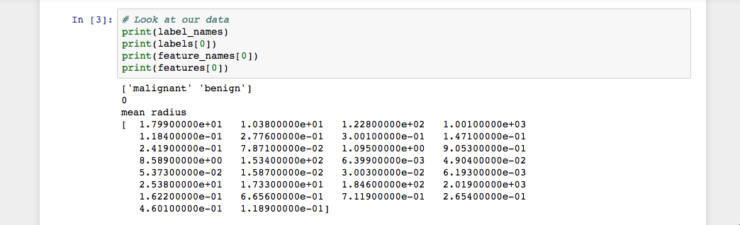
As the image shows, our class names are malignant and benign, which are then mapped to binary values of 0 and 1, where 0 represents malignant tumors and 1 represents benign tumors. Therefore, our first data instance is a malignant tumor whose mean radius is 1.79900000e+01.
Now that we have our data loaded, we can work with our data to build our machine learning classifier.
Step 3 — Organizing Data into Sets
To evaluate how well a classifier is performing, you should always test the model on unseen data. Therefore, before building a model, split your data into two parts: a training set and a test set.
You use the training set to train and evaluate the model during the development stage. You then use the trained model to make predictions on the unseen test set. This approach gives you a sense of the model’s performance and robustness.
Fortunately, sklearn has a function called train_test_split(), which divides your data into these sets. Import the function and then use it to split the data:
...
from sklearn.model_selection import train_test_split


# Split our data
train, test, train_labels, test_labels = train_test_split(features,
                                                          labels,
                                                          test_size=0.33,
                                                          random_state=42)
The function randomly splits the data using the test_size parameter. In this example, we now have a test set (test) that represents 33% of the original dataset. The remaining data (train) then makes up the training data. We also have the respective labels for both the train/test variables, i.e. train_labels and test_labels.
We can now move on to training our first model.
Step 4 — Building and Evaluating the Model
There are many models for machine learning, and each model has its own strengths and weaknesses. In this tutorial, we will focus on a simple algorithm that usually performs well in binary classification tasks, namely Naive Bayes (NB).
First, import the GaussianNB module. Then initialize the model with the GaussianNB() function, then train the model by fitting it to the data using gnb.fit():
...
from sklearn.naive_bayes import GaussianNB


# Initialize our classifier
gnb = GaussianNB()

# Train our classifier
model = gnb.fit(train, train_labels)
After we train the model, we can then use the trained model to make predictions on our test set, which we do using the predict() function. The predict() function returns an array of predictions for each data instance in the test set. We can then print our predictions to get a sense of what the model determined.
Use the predict() function with the test set and print the results:
...
# Make predictions
preds = gnb.predict(test)
print(preds)
Run the code and you’ll see the following results:
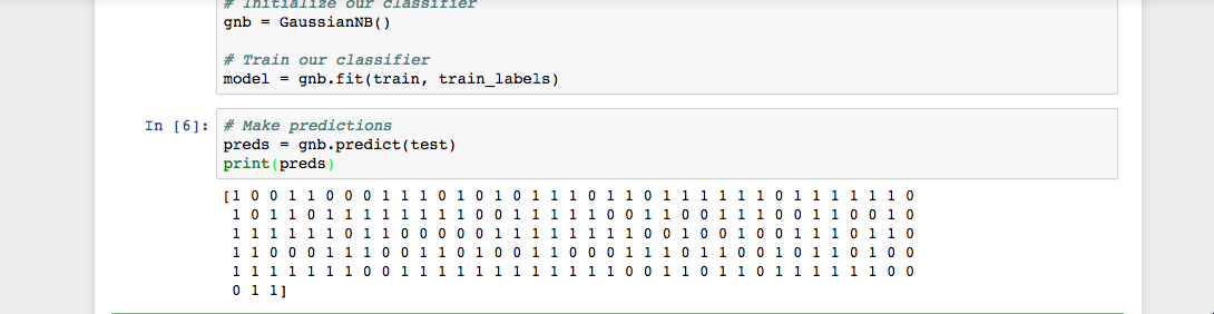
As you see in the Jupyter Notebook output, the predict() function returned an array of 0s and 1s which represent our predicted values for the tumor class (malignant vs. benign).
Now that we have our predictions, let’s evaluate how well our classifier is performing.
Step 5 — Evaluating the Model’s Accuracy
Using the array of true class labels, we can evaluate the accuracy of our model’s predicted values by comparing the two arrays (test_labels vs. preds). We will use the sklearn function accuracy_score() to determine the accuracy of our machine learning classifier.
...
from sklearn.metrics import accuracy_score


# Evaluate accuracy
print(accuracy_score(test_labels, preds))
You’ll see the following results:
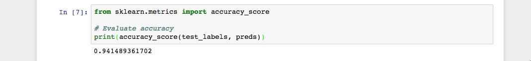
As you see in the output, the NB classifier is 94.15% accurate. This means that 94.15 percent of the time the classifier is able to make the correct prediction as to whether or not the tumor is malignant or benign. These results suggest that our feature set of 30 attributes are good indicators of tumor class.
You have successfully built your first machine learning classifier. Let’s reorganize the code by placing all import statements at the top of the Notebook or script. The final version of the code should look like this:
from sklearn.datasets import load_breast_cancer
from sklearn.model_selection import train_test_split
from sklearn.naive_bayes import GaussianNB
from sklearn.metrics import accuracy_score


# Load dataset
data = load_breast_cancer()

# Organize our data
label_names = data['target_names']
labels = data['target']
feature_names = data['feature_names']
features = data['data']

# Look at our data
print(label_names)
print('Class label = ', labels[0])
print(feature_names)
print(features[0])

# Split our data
train, test, train_labels, test_labels = train_test_split(features,
                                                          labels,
                                                          test_size=0.33,
                                                          random_state=42)

# Initialize our classifier
gnb = GaussianNB()

# Train our classifier
model = gnb.fit(train, train_labels)

# Make predictions
preds = gnb.predict(test)
print(preds)

# Evaluate accuracy
print(accuracy_score(test_labels, preds))
Now you can continue to work with your code to see if you can make your classifier perform even better. You could experiment with different subsets of features or even try completely different algorithms. Check out Scikit-learn’s website for more machine learning ideas.
Conclusion
In this tutorial, you learned how to build a machine learning classifier in Python. Now you can load data, organize data, train, predict, and evaluate machine learning classifiers in Python using Scikit-learn. The steps in this tutorial should help you facilitate the process of working with your own data in Python.
Thanks for learning with the DigitalOcean Community. Check out our offerings for compute, storage, networking, and managed databases.
About the author(s)
Managed the Write for DOnations program, wrote and edited community articles, and makes things on the Internet. Expertise in DevOps areas including Linux, Ubuntu, Debian, and more.
Still looking for an answer?
This textbox defaults to using Markdown to format your answer.
You can type !ref in this text area to quickly search our full set of tutorials, documentation & marketplace offerings and insert the link!
Thank you for this wonderful tutorial. but as a programmer, what comes next? I mean, what I would use for my program ? the training is the step to get the best parameters to use, the training step takes time, and the user will not stay everytime, he needs the best parameters to run the model, so how to do that?
Hello, good afternoon, I am new to this from the sklearn bookstore and I already studied the tutorial, very good the truth, but I want to know if after having our training set as I can make a prediction, how could a possible cancer enter and this one tell me Is it benign or malefic? That’s my question, how can I use the training set?
thank you very much for your attention.
Clear, easy to implement and follow . Thank you very much for such a great article.
Hello, I m very thankful for this wonderful tutorial. As a researcher, I want to ask how to load a dataset present as .csv file.
This tutorial is a solid introduction to building a machine learning classifier with Scikit-learn. I liked how it explains the complete workflow step by step, from loading the dataset and splitting training/testing data to training the model and measuring accuracy. Using a real dataset makes the concepts easier to understand, especially for beginners learning how classification works in practice. The examples are simple enough to follow without feeling overwhelming. One suggestion would be to briefly cover additional evaluation metrics like precision, recall, or confusion matrices, since accuracy alone may not always reflect model performance. Overall, it’s a helpful guide for anyone getting started with machine learning in Python.
 This work is licensed under a Creative Commons Attribution-NonCommercial- ShareAlike 4.0 International License.
Become a contributor for community
Get paid to write technical tutorials and select a tech-focused charity to receive a matching donation.

DigitalOcean Documentation
Full documentation for every DigitalOcean product.

Resources for startups and AI-native businesses
The Wave has everything you need to know about building a business, from raising funding to marketing your product.
The developer cloud
Scale up as you grow — whether you're running one virtual machine or ten thousand.

Start building today
From GPU-powered inference and Kubernetes to managed databases and storage, get everything you need to build, scale, and deploy intelligent applications.
