How to Evaluate Deep Learning Models: Key Metrics Explained

Introduction

In computer vision, object detection is the task of identifying and locating objects within an image. Whether it’s detecting cars on a road, people in a crowd, or products on a shelf, object detection helps machines “see” and understand visual data. Traditional techniques relied heavily on manual feature extraction and were often limited in accuracy. However, with the rise of deep learning, models like R-CNN and YOLO have significantly improved performance by learning features directly from the data.

These models take an image as input and return bounding boxes with class labels around each detected object, making them ideal for real-world applications like autonomous driving, surveillance, and medical imaging. While achieving good predictions is important, it’s just as critical to evaluate how well a model is performing. In this tutorial, we’ll walk through key evaluation metrics such as the confusion matrix, precision, recall, and accuracy—all of which help us understand the quality of predictions in object detection.

Let’s dive in and learn how to measure what really matters in object detection models.

Prerequisites

To follow along with this article, you will need experience with Python code and a basic understanding of Deep Learning. We will assume that all readers have access to sufficiently powerful machines so they can run the code provided. If you do not have access to a GPU, we suggest using DigitalOcean GPU Droplets. For instructions on getting started with Python code, we recommend the Python guide for beginners. This guide will help you set up your system and prepare to run beginner tutorials.

Confusion Matrix for Binary Classification

In binary classification, each input sample is assigned to one of two classes. Generally, these two classes are assigned labels like 1 and 0 or positive and negative. More specifically, the two class labels might be something like malignant or benign (e.g., if the problem concerns cancer classification) or success or failure (e.g., if it concerns classifying student test scores). Assume there is a binary classification problem with the classes positive and negative. Here are the labels for the seven samples used to train the model. These are called the sample’s ground-truth labels.

positive, negative, negative, positive, positive, positive, negative

Note that the class labels help us humans differentiate between the different classes. The thing that is of high importance to the model is a numeric score. When feeding a single sample to the model, the model does not necessarily return a class label but rather a score. For instance, when these seven samples are fed to the model, their class scores could be:

0.6, 0.2, 0.55, 0.9, 0.4, 0.8, 0.5

Based on the scores, each sample is given a class label. How do we convert these scores into labels? We do this by using a threshold. This threshold is a hyperparameter of the model and can be defined by the user. For example, the threshold could be 0.5–then any sample above or equal to 0.5 is given the positive label. Otherwise, it is negative. Here are the predicted labels for the samples:

positive (0.6), negative (0.2), positive (0.55), positive (0.9), negative (0.4), positive (0.8), positive (0.5)

For comparison, here are both the ground truth and predicted labels. At first glance, we can see 4 correct and 3 incorrect predictions. Note that changing the threshold might give different results. For example, setting the threshold to 0.6 leaves only two incorrect predictions.

Ground-Truth: positive, negative, negative, positive, positive, positive, negative
Predicted   : positive, negative, positive, positive, negative, positive, positive

A confusion matrix is used to extract more information about model performance. It helps us visualize whether the model is “confused” in discriminating between the two classes. As seen in the next figure, it is a 2×2 matrix. The labels of the two rows and columns are Positive and Negative to reflect the two class labels. In this example, the row labels represent the ground-truth labels, while the column labels represent the predicted labels. This could be changed.

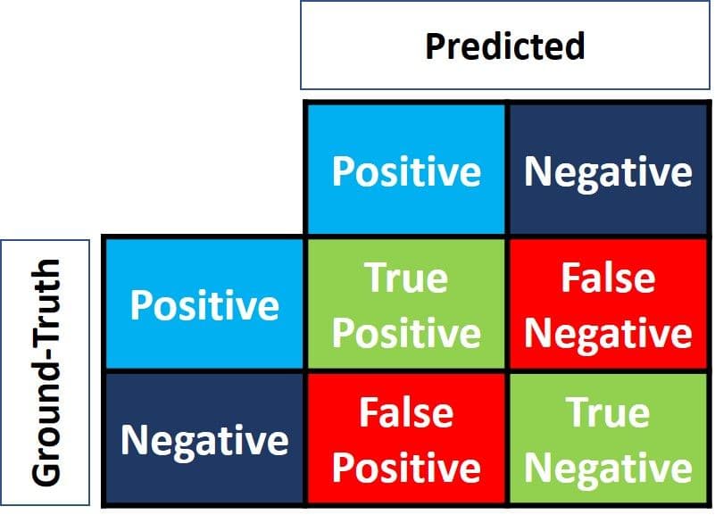
The 4 elements of the matrix (the items in red and green) represent the 4 metrics that count the number of correct and incorrect predictions the model made. Each element is given a label that consists of two words:

1. True or False
2. Positive or Negative

It is True when the prediction is correct (i.e., a match between the predicted and ground-truth labels) and False when there is a mismatch between the predicted and ground-truth labels. Positive or Negative refers to the predicted label.

In summary, the first word is False whenever the prediction is wrong. Otherwise, it is True. The goal is to maximize the metrics with the word True (True Positive and True Negative), and minimize the other two metrics (False Positive and False Negative). The four metrics in the confusion matrix are thus:

1. Top-Left (True Positive): How many times did the model correctly classify a Positive sample as Positive?
2. Top-Right (False Negative): How often did the model incorrectly classify a Positive sample as Negative?
3. Bottom-Left (False Positive): How many times did the model incorrectly classify a Negative sample as Positive?
4. Bottom-Right (True Negative): How many times did the model correctly classify a Negative sample as Negative?

We can calculate these four metrics for the seven predictions we saw previously. The resulting confusion matrix is given in the next figure.

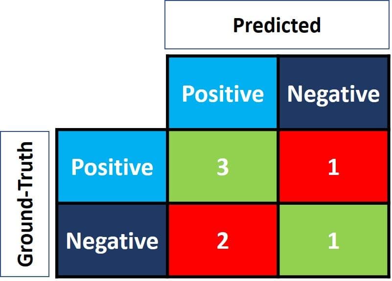
This is how the confusion matrix is calculated for a binary classification problem. Now let’s see how it would be calculated for a multi-class problem.

Confusion Matrix for Multi-Class Classification

What if we have more than two classes? How do we calculate these four metrics in the confusion matrix for a multi-class classification problem? Simple!

Assume there are 9 samples, where each sample belongs to one of three classes: White, Black, or Red. Here is the ground-truth data for the 9 samples.

Red, Black, Red, White, White, Red, Black, Red, White

When the samples are fed into a model, here are the predicted labels.

Red, White, Black, White, Red, Red, Black, White, Red

For easier comparison, here they are side-by-side.

Ground-Truth: Red, Black, Red,   White, White, Red, Black, Red,   White
Predicted:    Red, White, Black, White, Red,   Red, Black, White, Red

Before calculating the confusion matrix, a target class must be specified. Let’s set the Red class as the target. This class is marked as Positive, and all other classes are marked as Negative.

Positive, Negative, Positive, Negative, Negative, Positive, Negative, Positive, Negative
Positive, Negative, Negative, Negative, Positive, Positive, Negative, Negative, Positive

There are now only two classes again (Positive and Negative). Thus, the confusion matrix can be calculated as in the previous section. Note that this matrix is just for the Red class.

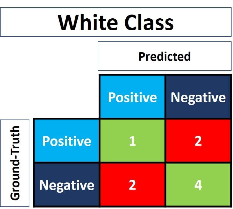
For the White class, replace each of its occurrences as Positive and all other class labels as Negative. After replacement, here are the ground-truth and predicted labels. The next figure shows the confusion matrix for the White class.

Negative, Negative, Negative, Positive, Positive, Negative, Negative, Negative, Positive
Negative, Positive, Negative, Positive, Negative, Negative, Negative, Positive, Negative

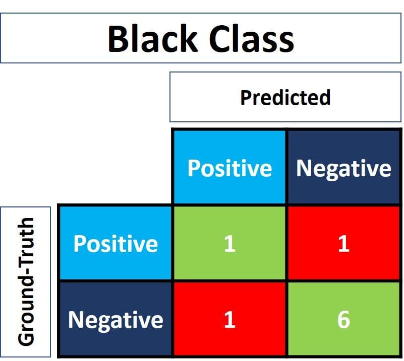
Similarly, here is the confusion matrix for the Black class.

Calculating the Confusion Matrix with Scikit-Learn

The popular Scikit-learn library in Python has a module called metrics that can calculate the metrics in the confusion matrix.

For binary-class problems, the confusion_matrix() function is used. Among its accepted parameters, we use these two:

1. y_true: The ground-truth labels.
2. y_pred: The predicted labels.

The following code calculates the confusion matrix for the previously discussed binary classification example.

import sklearn.metrics

y_true = ["positive", "negative", "negative", "positive", "positive", "positive", "negative"]
y_pred = ["positive", "negative", "positive", "positive", "negative", "positive", "positive"]

r = sklearn.metrics.confusion_matrix(y_true, y_pred)
print(r)

array([[1, 2],
      [1, 3]], dtype=int64)

Note that the order of the metrics differs from that discussed previously. For example, the True Positive metric is at the bottom-right corner while the True Negative is at the top-left corner. To fix that, we can flip the matrix.

import numpy

r = numpy.flip(r)
print(r)

array([[3, 1],
       [2, 1]], dtype=int64)

The multilabel_confusion_matrix () function is used to calculate the confusion matrix for a multi-class classification problem, as shown below. In addition to the y_true and y_pred parameters, a third parameter named labels accepts a list of the class labels.

import sklearn.metrics
import numpy

y_true = ["Red", "Black", "Red",   "White", "White", "Red", "Black", "Red",   "White"]
y_pred = ["Red", "White", "Black", "White", "Red",   "Red", "Black", "White", "Red"]

r = sklearn.metrics.multilabel_confusion_matrix(y_true, y_pred, labels=["White", "Black", "Red"])
print(r)

array([
      [[4 2]
      [2 1]]

       [[6 1]
        [1 1]]

        [[3 2]
         [2 2]]], dtype=int64)

The function calculates the confusion matrix for each class and returns all the matrices. The order of the matrices matches the order of the labels in the labels parameter. To adjust the order of the metrics in the matrices, we’ll use numpy.flip() function, as before.

print(numpy.flip(r[0])) # White class confusion matrix
print(numpy.flip(r[1])) # Black class confusion matrix
print(numpy.flip(r[2])) # Red class confusion matrix

# White class confusion matrix
[[1 2]
  [2 4]]

# Black class confusion matrix
[[1 1]
  [1 6]]

# Red class confusion matrix
[[2 2]
  [2 3]]

In the rest of this tutorial, we’ll focus on just two classes. The next section discusses three key metrics calculated using the confusion matrix.

Accuracy, Precision, and Recall

The confusion matrix offers four different and individual metrics, as we’ve already seen. Based on these four metrics, other metrics can be calculated that offer more information about how the model behaves:

1. Accuracy
2. Precision
3. Recall

The next subsections discuss each of these three metrics.

Accuracy

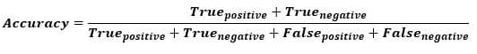
Accuracy is a metric that generally describes how the model performs across all classes. It is useful when all classes are of equal importance. It is calculated as the ratio between the number of correct predictions and the total number of predictions.

Here is how to calculate the accuracy using Scikit-learn, based on the confusion matrix previously calculated. The variable acc holds the result of dividing the sum of True Positives and True Negatives by the sum of all values in the matrix. The result is 0.5714, which means the model is 57.14% accurate in making a correct prediction.

import numpy
import sklearn.metrics

y_true = ["positive", "negative", "negative", "positive", "positive", "positive", "negative"]
y_pred = ["positive", "negative", "positive", "positive", "negative", "positive", "positive"]

r = sklearn.metrics.confusion_matrix(y_true, y_pred)

r = numpy.flip(r)

acc = (r[0][0] + r[-1][-1]) / numpy.sum(r)
print(acc)

0.571

The sklearn. metrics module has a function called accuracy_score() that can also calculate the accuracy. It accepts the ground-truth and predicted labels as arguments.

acc = sklearn.metrics.accuracy_score(y_true, y_pred)

Note that the accuracy may be deceptive. One case is when the data is imbalanced. Assume there are 600 samples, where 550 belong to the Positive class and just 50 to the Negative class. Since most of the samples belong to one class, the accuracy for that class will be higher than for the other.

If the model made 530/550 correct predictions for the Positive class, compared to just 5/50 for the Negative class, then the total accuracy is (530 + 5) / 600 = 0.8917. This means the model is 89.17% accurate. With that in mind, for any sample (regardless of its class), the model will likely make a correct prediction 89.17% of the time. This is not valid, especially when considering the Negative class for which the model performed badly.

Precision

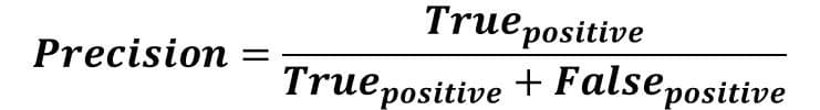
The precision is calculated as the ratio between the number of Positive samples correctly classified to the total number of samples classified as Positive (either correctly or incorrectly). The precision measures the model’s accuracy in classifying a sample as positive.

When the model makes many incorrect Positive or few correct Positive classifications, this increases the denominator and makes the precision small. On the other hand, the precision is high when:

1. The model makes many correct Positive classifications (maximizes True positives).
2. The model makes fewer incorrect Positive classifications (minimizes False positives).

Imagine a man trusted by others; when he predicts something, others believe him. The precision is like this man. When the precision is high, you can trust the model when it predicts a sample as Positive. Thus, precision helps to know how accurate the model is when it says a sample is positive.

Now, let us understand what Precision is.

The precision reflects how reliably the model is in classifying samples as Positive.

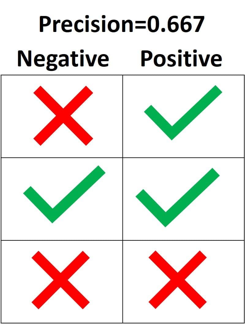
In the next figure, the green mark means a sample is classified as Positive and a red mark means the sample is Negative. The model correctly classified two Positive samples, but incorrectly classified one Negative sample as Positive. Thus, the True Positive rate is 2 and the False Positive rate is 1, and the precision is 2/(2+1)=0.667. In other words, the trustworthiness percentage of the model when it says that a sample is Positive is 66.7%.

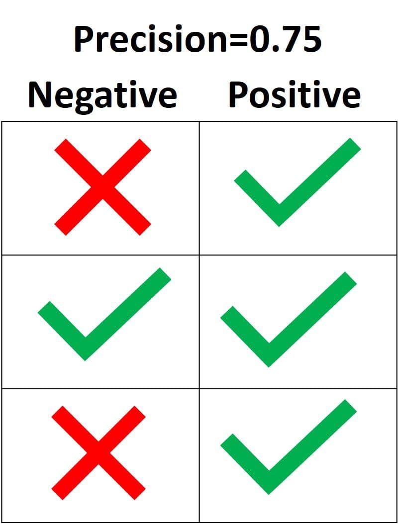
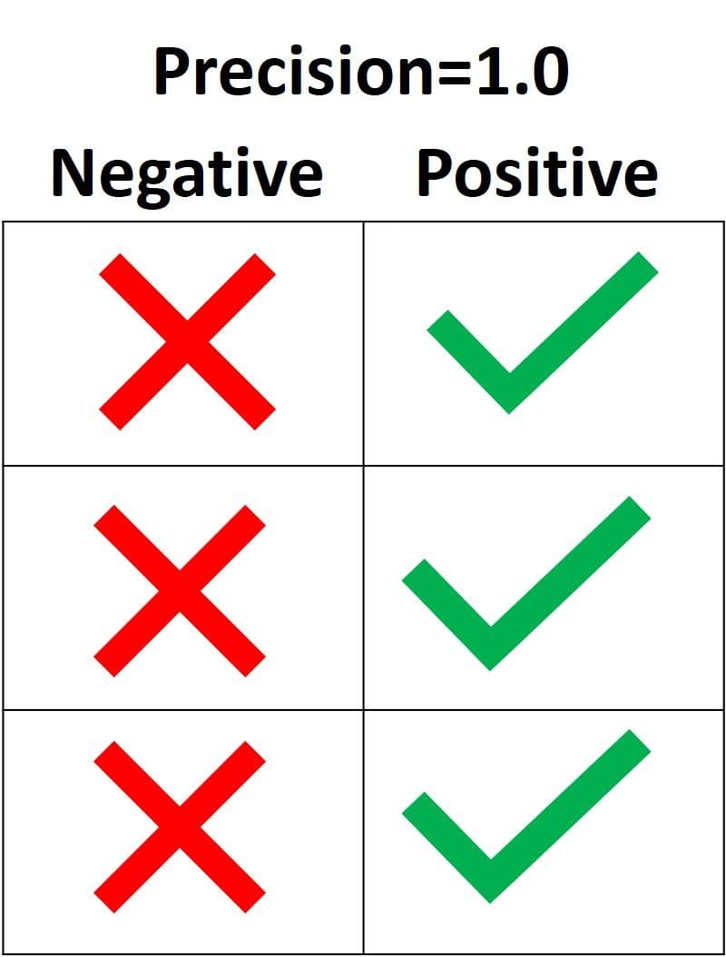
The goal of the precision is to classify all the Positive samples as Positive, and not misclassify a negative sample as Positive. According to the next figure, if all three Positive samples are correctly classified but one Negative sample is incorrectly classified, the precision is 3/(3+1)=0.75. Thus, the model is 75% accurate when it says that a sample is positive.

The only way to get 100% precision is to classify all the Positive samples as Positive, in addition to not misclassifying a Negative sample as Positive.

In Scikit-learn, the sklearn.The metrics module has a function named precision_score(), which accepts the ground-truth and predicted labels and returns the precision. The pos_label parameter accepts the label of the Positive class. It defaults to 1.

import sklearn.metrics

y_true = ["positive", "positive", "positive", "negative", "negative", "negative"]
y_pred = ["positive", "positive", "negative", "positive", "negative", "negative"]

precision = sklearn.metrics.precision_score(y_true, y_pred, pos_label="positive")
print(precision)

0.6666666666666666

Recall

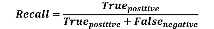
The recall is calculated as the ratio between the number of Positive samples correctly classified as Positive to the total number of Positive samples. The recall measures the model’s ability to detect Positive samples. The higher the recall, the more positive samples detected.

The recall cares only about how the positive samples are classified. This is independent of how the negative samples are classified, e.g., for the precision. When the model classifies all the positive samples as Positive, then the recall will be 100% even if all the negative samples were incorrectly classified as Positive. Let’s look at some examples.

In the next figure, there are 4 different cases (A to D), and all have the same recall which is 0.667. Each case differs only in how the negative samples are classified. For example, case A has all the negative samples correctly classified as Negative, but case D misclassifies all the negative samples as Positive. Independent of how the negative samples are classified, the recall only cares about the positive samples.

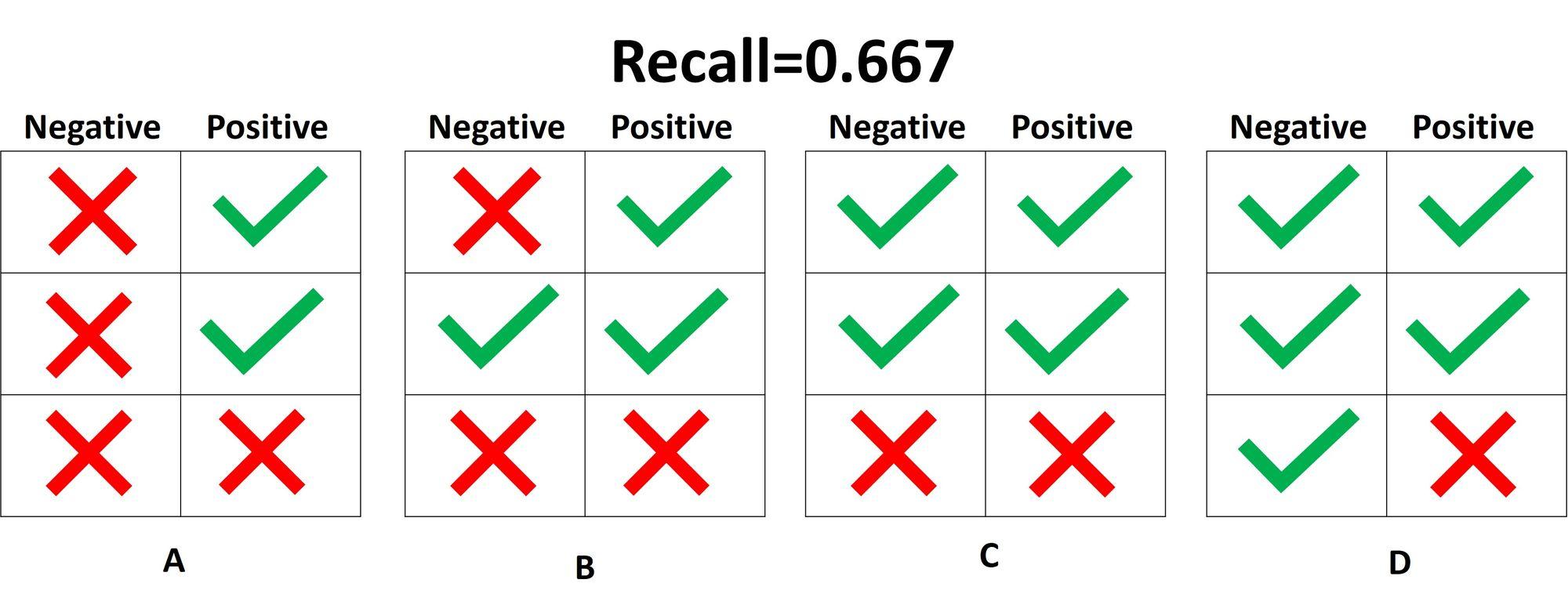
Out of the 4 cases shown above, only 2 positive samples are classified correctly as positive. Thus, the True Positive rate is 2. The False Negative rate is 1 because just a single positive sample is classified as negative. As a result, the recall is 2/(2+1)=2/3=0.667.

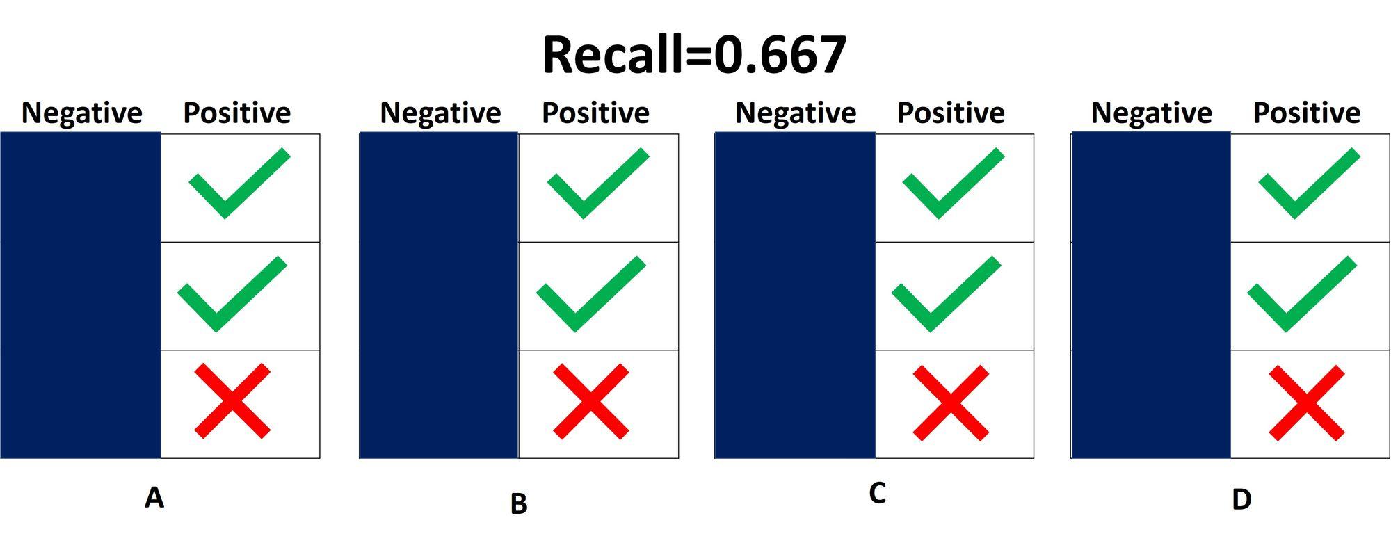
Because it does not matter whether the negative samples are classified as positive or negative, it is better to neglect the negative samples altogether as shown in the next figure. You only need to consider the positive samples when calculating the recall.

What does it mean when the recall is high or low? When the recall is high, it means the model can classify all the positive samples correctly as Positive. Thus, the model can be trusted in its ability to detect positive samples.

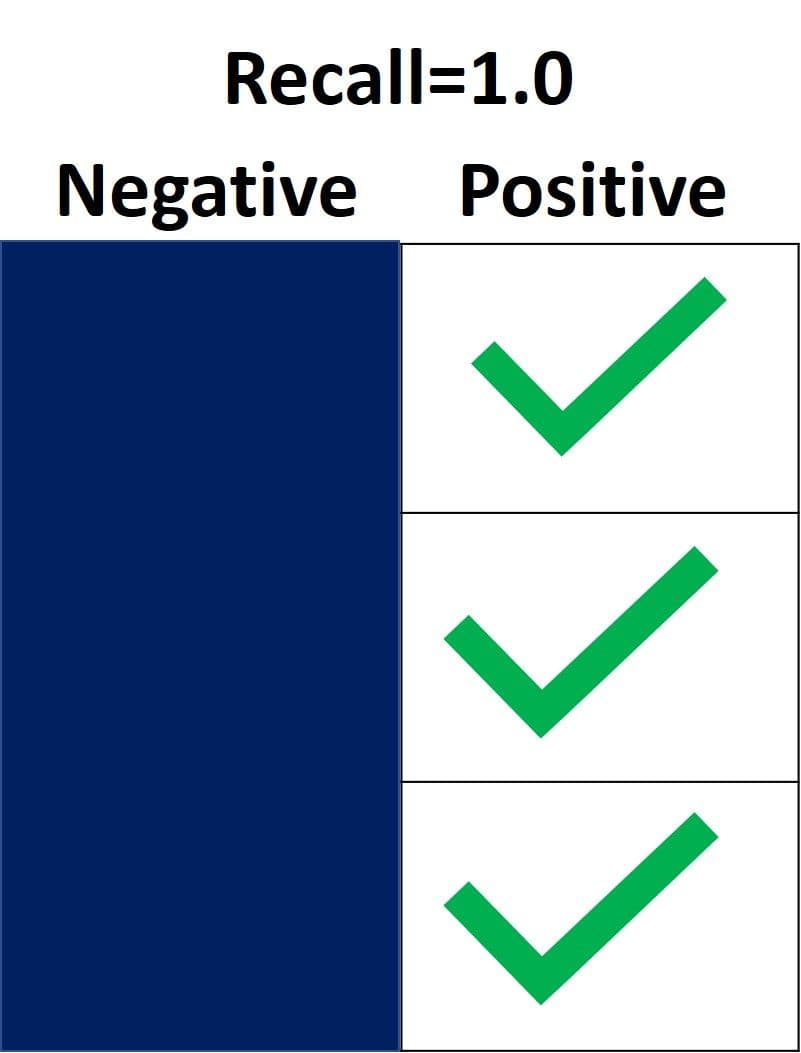
In the next figure, the recall is 1.0 because all the positive samples were correctly classified as Positive. The True Positive rate is 3, and the False Negative rate is 0. Thus, the recall is equal to 3/(3+0)=1. This means the model detected all the positive samples. Because the recall neglects how the negative samples are classified, there could still be many negative samples classified as positive (i.e., a high False Positive rate). The recall doesn’t take this into account.

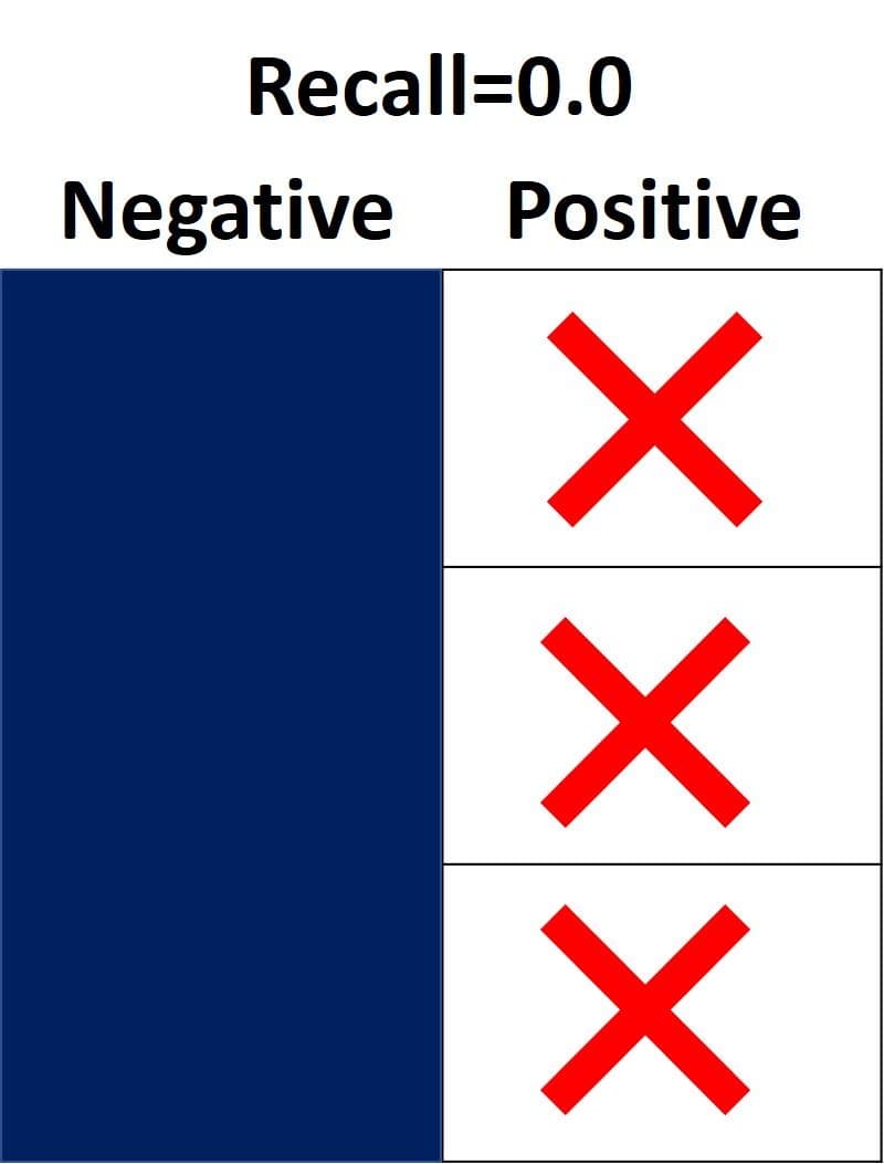
On the other hand, the recall is 0.0 when it fails to detect any positive sample. In the next figure, all the positive samples are incorrectly classified as Negative. This means the model detected 0% of the positive samples. The True Positive rate is 0, and the False Negative rate is 3. Thus, the recall is equal to 0/(0+3)=0.

When the recall has a value between 0.0 and 1.0, this value reflects the percentage of positive samples the model correctly classified as Positive. For example, if there are 10 positive samples and the recall is 0.6, this means the model correctly classified 60% of the positive samples (i.e., 0.6*10=6 positive samples are correctly classified).

Similar to the precision_score() function, the recall_score() function in the sklearn.metrics module calculates the recall. The next block of code shows an example.

import sklearn.metrics

y_true = ["positive", "positive", "positive", "negative", "negative", "negative"]
y_pred = ["positive", "positive", "negative", "positive", "negative", "negative"]

recall = sklearn.metrics.recall_score(y_true, y_pred, pos_label="positive")
print(recall)

0.6666666666666666

After defining both the precision and the recall, let’s have a quick recap:

1. The precision measures the model’s trustworthiness in classifying positive samples, and the recall measures how many positive samples the model correctly classified.
2. The precision considers how the positive and negative samples were classified, but the recall only considers the positive samples in its calculations. In other words, the precision depends on both the negative and positive samples, but the recall is dependent only on the positive samples (and independent of the negative samples).
3. The precision considers when a sample is classified as Positive, but it does not consider correctly classifying all positive samples. The recall cares about correctly classifying all positive samples, but it does not care if a negative sample is classified as positive.
4. When a model has high recall but low precision, it classifies most of the positive samples correctly but has many false positives (i.e., it classifies many Negative samples as Positive). When a model has high precision but low recall, it is accurate when it classifies a sample as Positive, but can only classify a few positive samples.

Here are some questions to test your understanding:

1. If the recall is 1.0 and the dataset has 5 positive samples, how many positive samples were correctly classified by the model? (5)
2. Given that the recall is 0.3 when the dataset has 30 positive samples, how many positive samples were correctly classified by the model? (0.3*30=9 samples)
3. If the recall is 0.0 and the dataset has 14 positive samples, how many positive samples were correctly classified by the model? (0)

Precision or Recall?

The decision of whether to use precision or recall depends on the type of problem being solved. If the goal is to detect all the positive samples (without caring whether negative samples would be misclassified as positive), then use recall. Use precision if the problem is sensitive to classifying a sample as Positive in general, i.e., including Negative samples that were falsely classified as Positive.

Imagine being given an image and asked to detect all the cars within it. Which metric do you use? The goal is to detect all the cars and use a recall. This may misclassify some objects as cars, but it will eventually work towards detecting all the target objects.

Now, say you’re given a mammography image, and you are asked to detect whether there is cancer or not. Which metric do you use? Because it is sensitive to incorrectly identifying an image as cancerous, we must be sure when classifying an image as Positive (i.e., has cancer). Thus, precision is the preferred metric.

FAQ’s

1. What is a confusion matrix in deep learning?

A confusion matrix is a table that summarizes the performance of a classification model by comparing predicted and actual labels. It provides insights into which classes are being correctly or incorrectly predicted.

2. How is accuracy calculated in a classification model?

Accuracy = (True Positives + True Negatives) / (Total Samples). It gives a general idea of how often the model is correct, but may not reflect class-wise performance.

3. What is the difference between precision and recall?

Precision measures correctness among positive predictions, while recall measures how many actual positives were identified.Both are crucial for understanding how a model performs, especially with imbalanced datasets.

4. When should I prioritize precision over recall?

Prioritize precision when false positives are costly, such as in medical diagnosis or fraud detection. High precision ensures that positive predictions are reliable and trustworthy.

5. How do I calculate the confusion matrix in Python using Scikit-learn?

Use from sklearn.metrics import confusion_matrix; confusion_matrix(y_true, y_pred).This function returns a matrix you can use to calculate other evaluation metrics.

6. How does the confusion matrix apply to multi-class classification?

It extends to multi-class problems by creating an NxN matrix where N is the number of classes.Each cell in the matrix shows how frequently a specific class was predicted versus the actual class.

7. What are true positives, false positives, true negatives, and false negatives?

• True Positive (TP): Correctly predicted positive cases.
• False Positive (FP): Incorrectly predicted positive cases.
• True Negative (TN): Correctly predicted negative cases.
• False Negative (FN): Incorrectly predicted negative cases.

Understanding these values is essential for computing metrics like precision and recall.

8. How do accuracy, precision, and recall impact model performance?

They determine how well a model balances correct predictions, minimizing false positives and false negatives. A well-performing model should aim for high values across all three metrics.

9. Why is accuracy sometimes misleading as an evaluation metric?

Accuracy can be misleading in imbalanced datasets where one class dominates predictions. In such cases, precision, recall, or F1-score provide a more realistic evaluation.

10. How do I interpret a confusion matrix for an object detection model?

A confusion matrix is a table that summarizes how well a classification model performs, for both binary and multi-class tasks. It shows correct predictions (true positives and true negatives) and errors (false positives and false negatives), which help calculate metrics like precision and recall.

11. What are the common challenges when evaluating deep learning models?

Handling class imbalance, overfitting, data quality issues, and selecting the right evaluation metrics. Overcoming these challenges often requires a combination of data engineering and model tuning.

12. How can I improve the precision and recall of my model?

Use better data preprocessing, adjust classification thresholds, tune hyperparameters, and apply data augmentation. You can also try using more advanced architectures or adding more labeled data.

13. What is the role of a confusion matrix in object detection tasks?

It helps analyze detection errors, including misclassifications, missed detections, and false alarms. Combined with IoU and mAP, it offers a comprehensive evaluation framework for object detectors.

Conclusion

In this tutorial, we explored how confusion matrices help evaluate the performance of classification models in both binary and multi-class scenarios. We broke down the four essential metrics—true positives, false positives, true negatives, and false negatives—and showed how they contribute to computing accuracy, precision, and recall. Using Python’s scikit-learn library, we demonstrated how to easily generate and interpret these metrics in real-world use cases.

Understanding these evaluation metrics is critical for building robust deep learning models, especially in domains like healthcare, finance, and autonomous systems where the cost of errors can be high. Whether you’re just starting with machine learning or scaling your projects into production, keeping a close eye on these metrics will help you fine-tune model performance effectively.

If you’re looking to train and deploy deep learning models efficiently, consider using DigitalOcean’s GPU-accelerated Droplets. These tools provide powerful compute infrastructure to run your experiments, monitor performance, and scale with ease.

Happy modeling—and don’t forget, understanding your model is just as important as building it!

References

1. Understanding Model Evaluation Metrics - Scikit-learn Documentation
2. Accuracy, Precision, and Recall Explained - DigitalOcean Blog
3. Confusion Matrix for Model Performance Analysis - Towards DataScience Blog
4. Optimizing Deep Learning Model Performance - DigitalOcean Blog
5. Hyperparameter Tuning for Better Model Metrics - DigitalOcean Blog
6. Measuring Object Detection Model Performance - Papers With Code