Dropout Regularization in Deep Learning

One of the major problems with deep learning networks is that as the neural network keeps getting denser and denser, it faces the issue known as overfitting. Underfitting will never occur with a multi-layered deep neural network; however, there is always a possibility of overfitting. This is because, as the neural network becomes more and more complex, the weights of every neuron try to fit the data well. A machine learning model or a Deep learning model that fits the training data well, but fails to perform well with unseen data, this phenomenon is known as overfitting. Further, underfitting is a phenomenon when the model performs poorly on both training and test data.

Among various regularization techniques, Dropout is a simple yet highly effective method that helps overcome overfitting. In our previous articles, we have already discussed regularization techniques such as Ridge and Lasso. This article explores dropout regularization, how it works, and why it’s a powerful tool for training deep learning models.

Dropout is a regularization technique where, during the training phase, a subset of neurons is deactivated randomly or “dropped out” or ignored in each forward and backward pass. This number is decided by something called the dropout ratio, which we will discuss soon in this article. Formally, given a layer with n neurons, dropout randomly sets a fraction of them to zero during training. These neurons do not contribute to the forward pass nor participate in backpropagation. The idea was introduced in the paper by Srivastava et al. (2014), the Dropout paper, under the supervision of Geoffrey Hinton. Dropout is very similar to Random Forests, as in both cases, there is a random selection of either features or neurons. Random Forest also randomly selects features/trees and reduces overfitting, thus increasing model robustness.

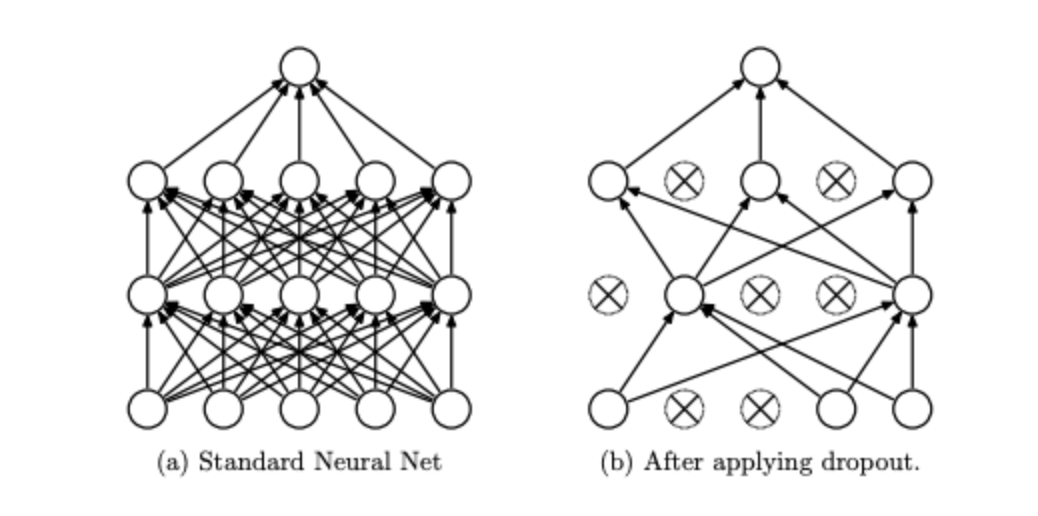
(Image Source: Original Research Paper)

As a neural network becomes deeper and deeper, there is a chance that the parameters tend to memorize the training dataset so well that it leads to poor generalization on new, unseen datasets, causing high variance. Hence, a regularization technique such as Dropout is a simple and effective way to maintain the balance of bias and variance. Hence, building a model that performs well on unseen data as well. This process stops the network from over-relying on particular neurons. The network learns to rely on stronger features that don’t depend too much on any single neuron.

The dropout ratio (often denoted as *p*) refers to the fraction of neurons that are randomly deactivated during the training phase. For example, if the dropout ratio is r=0.5, it means that 50% of the neurons are turned off in each training iteration. However, there are no fixed rules to select this ratio, but some of the common approaches are discussed below:

1. Start with Common Defaults:
   • Input layer: 0.1–0.2 (lower to avoid losing too much raw data).
   • Hidden layers: 0.3–0.5 (moderate dropout to encourage robustness).
   • Output layer: Often no dropout (to preserve final predictions).
2. Grid Search or Random Search:
   • Test different values (e.g., 0.1, 0.3, 0.5) and compare validation performance.
3. Monitor Overfitting:
   • If the model overfits (high training accuracy but low validation accuracy), increase dropout.
   • If the model underfits (poor training accuracy), reduce dropout.
4. Layer-Specific Adjustments:
   • Deeper layers may need higher dropout (since they tend to overfit more).
5. Observations:
   • CNNs often use 0.2–0.5. (Dropout may not be useful for convolutional layers in some cases, but can be effective in fully connected layers.)
   • RNNs/LSTMs use 0.1–0.3 (since sequential data is more sensitive).

Here is an example code:

from tensorflow.keras.models import Sequential
from tensorflow.keras.layers import Dense, Dropout

model = Sequential([
    Dense(128, activation='relu', input_shape=(input_dim,)),
    Dropout(0.5),  # 50% dropout rate
    Dense(64, activation='relu'),
    Dropout(0.3),  # 30% dropout rate
    Dense(10, activation='softmax')
])

Some of the most common values usually range from 0.1 to 0.5, but experimentation is the key here.

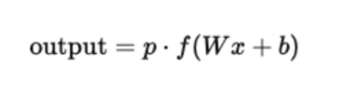
Now, as we learned earlier, during the training phase, Dropout randomly removes neurons, and this is done using the famous Bernoulli distribution. We will discuss the Bernoulli distribution in our upcoming articles in more detail. During the testing phase, the full network is connected, there are no activated and deactivated neurons, and the outputs are scaled by the dropout probability p to match the expected value during training. Mathematically: If dropout ratio = r, and keep probability = p, then during testing:

Now, we understand that dropout helps combat overfitting, but let us understand different points on how dropouts do this:

1. Stochastic training: Each iteration trains on a different network, thus reducing reliance on specific paths.
2. Model averaging: The final model behaves like a random forest model or an ensemble of several sub-networks.
3. Redundant representations: Dropout encourages the model to learn features that are useful across different combinations of neurons.

This leads to a simpler, more generalized model capable of performing better on unseen data.

Here’s a simple code example that demonstrates how Dropout works in a neural network:

import torch
import torch.nn as nn
import torch.optim as optim
from torchvision import datasets, transforms
from torch.utils.data import DataLoader

# Set seed for reproducibility
torch.manual_seed(42)

# Define transform for MNIST
transform = transforms.Compose([transforms.ToTensor(), transforms.Normalize((0.5,), (0.5,))])

# Load training and test data
train_dataset = datasets.MNIST(root='./data', train=True, download=True, transform=transform)
test_dataset  = datasets.MNIST(root='./data', train=False, download=True, transform=transform)

train_loader = DataLoader(train_dataset, batch_size=64, shuffle=True)
test_loader  = DataLoader(test_dataset, batch_size=1000, shuffle=False)

# Define model without dropout
class NoDropoutNet(nn.Module):
   def __init__(self):
       super(NoDropoutNet, self).__init__()
       self.fc1 = nn.Linear(784, 256)
       self.fc2 = nn.Linear(256, 128)
       self.fc3 = nn.Linear(128, 10)

   def forward(self, x):
       x = x.view(-1, 784)
       x = torch.relu(self.fc1(x))
       x = torch.relu(self.fc2(x))
       x = self.fc3(x)
       return x

# Define model with dropout
class DropoutNet(nn.Module):
   def __init__(self):
       super(DropoutNet, self).__init__()
       self.fc1 = nn.Linear(784, 256)
       self.dropout1 = nn.Dropout(0.5)
       self.fc2 = nn.Linear(256, 128)
       self.dropout2 = nn.Dropout(0.3)
       self.fc3 = nn.Linear(128, 10)

   def forward(self, x):
       x = x.view(-1, 784)
       x = torch.relu(self.fc1(x))
       x = self.dropout1(x)
       x = torch.relu(self.fc2(x))
       x = self.dropout2(x)
       x = self.fc3(x)
       return x

# Training function
def train(model, device, train_loader, optimizer, epoch):
   model.train()
   for batch_idx, (data, target) in enumerate(train_loader):
       data, target = data.to(device), target.to(device)
       optimizer.zero_grad()
       output = model(data)
       loss = nn.CrossEntropyLoss()(output, target)
       loss.backward()
       optimizer.step()

# Test function
def test(model, device, test_loader):
   model.eval()
   correct = 0
   with torch.no_grad():
       for data, target in test_loader:
           data, target = data.to(device), target.to(device)
           output = model(data)
           pred = output.argmax(dim=1)
           correct += pred.eq(target).sum().item()
   return correct / len(test_loader.dataset)

# Set device
device = torch.device("cuda" if torch.cuda.is_available() else "cpu")

# Train both models
models = {
   "No Dropout": NoDropoutNet().to(device),
   "With Dropout": DropoutNet().to(device)
}

for name, model in models.items():
   optimizer = optim.Adam(model.parameters())
   print(f"\nTraining {name} model...")
   for epoch in range(1, 6):  # 5 epochs
       train(model, device, train_loader, optimizer, epoch)
       acc = test(model, device, test_loader)
       print(f"Epoch {epoch}: Test Accuracy: {acc:.4f}")

100%|██████████| 9.91M/9.91M [00:01<00:00, 5.49MB/s]
100%|██████████| 28.9k/28.9k [00:00<00:00, 160kB/s]
100%|██████████| 1.65M/1.65M [00:01<00:00, 1.52MB/s]
100%|██████████| 4.54k/4.54k [00:00<00:00, 6.81MB/s]
Training No Dropout model…
Epoch 1: Test Accuracy: 0.9443
Epoch 2: Test Accuracy: 0.9623
Epoch 3: Test Accuracy: 0.9622
Epoch 4: Test Accuracy: 0.9697
Epoch 5: Test Accuracy: 0.9626

Training With Dropout model…
Epoch 1: Test Accuracy: 0.9351
Epoch 2: Test Accuracy: 0.9502
Epoch 3: Test Accuracy: 0.9541
Epoch 4: Test Accuracy: 0.9562
Epoch 5: Test Accuracy: 0.9632

import matplotlib.pyplot as plt

# Modified training and test functions to record accuracy
def train_and_evaluate(model, name, epochs=5):
   model.to(device)
   optimizer = optim.Adam(model.parameters())
   train_acc = []
   test_acc = []

   for epoch in range(epochs):
       model.train()
       correct_train = 0
       total_train = 0

       for data, target in train_loader:
           data, target = data.to(device), target.to(device)
           optimizer.zero_grad()
           output = model(data)
           loss = nn.CrossEntropyLoss()(output, target)
           loss.backward()
           optimizer.step()
           pred = output.argmax(dim=1)
           correct_train += pred.eq(target).sum().item()
           total_train += target.size(0)

       model.eval()
       correct_test = 0
       with torch.no_grad():
           for data, target in test_loader:
               data, target = data.to(device), target.to(device)
               output = model(data)
               pred = output.argmax(dim=1)
               correct_test += pred.eq(target).sum().item()

       train_accuracy = correct_train / total_train
       test_accuracy = correct_test / len(test_loader.dataset)
       train_acc.append(train_accuracy)
       test_acc.append(test_accuracy)

       print(f"{name} - Epoch {epoch+1}: Train Acc = {train_accuracy:.4f}, Test Acc = {test_accuracy:.4f}")

   return train_acc, test_acc

model1 = NoDropoutNet()
model2 = DropoutNet()

train_acc1, test_acc1 = train_and_evaluate(model1, "No Dropout")
train_acc2, test_acc2 = train_and_evaluate(model2, "With Dropout")

No Dropout - Epoch 1: Train Acc = 0.8982, Test Acc = 0.9396
No Dropout - Epoch 2: Train Acc = 0.9555, Test Acc = 0.9613
No Dropout - Epoch 3: Train Acc = 0.9645, Test Acc = 0.9653
No Dropout - Epoch 4: Train Acc = 0.9723, Test Acc = 0.9707
No Dropout - Epoch 5: Train Acc = 0.9757, Test Acc = 0.9719
With Dropout - Epoch 1: Train Acc = 0.8306, Test Acc = 0.9366
With Dropout - Epoch 2: Train Acc = 0.9028, Test Acc = 0.9500
With Dropout - Epoch 3: Train Acc = 0.9142, Test Acc = 0.9515
With Dropout - Epoch 4: Train Acc = 0.9231, Test Acc = 0.9559
With Dropout - Epoch 5: Train Acc = 0.9269, Test Acc = 0.9586

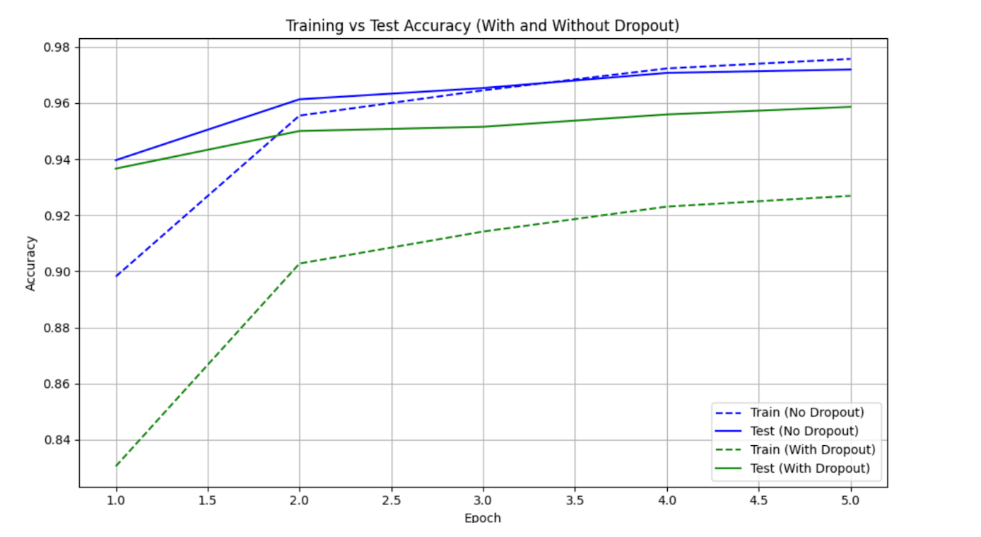
# Plotting accuracy comparison
plt.figure(figsize=(10, 6))
epochs = range(1, 6)

plt.plot(epochs, train_acc1, label='Train (No Dropout)', linestyle='--', color='blue')
plt.plot(epochs, test_acc1, label='Test (No Dropout)', color='blue')

plt.plot(epochs, train_acc2, label='Train (With Dropout)', linestyle='--', color='green')
plt.plot(epochs, test_acc2, label='Test (With Dropout)', color='green')

plt.xlabel('Epoch')
plt.ylabel('Accuracy')
plt.title('Training vs Test Accuracy (With and Without Dropout)')
plt.legend()
plt.grid(True)
plt.tight_layout()
plt.show()

You can train this model using MNIST or any image dataset.

The Dropout layers are only active during training (model.train()) and automatically disabled during inference (model.eval()). You can experiment with p-values in nn.Dropout(p=…) to observe the effect of different dropout ratios. Adding a Dropout to a model might learn slightly slower, but often generalizes better, showing improved test performance.

1. What is a dropout layer?

A dropout layer is a tool used in neural networks to prevent overfitting. During training, it randomly turns off some neurons so the model doesn’t rely too much on any one part. This helps the network learn more general patterns that work better on new data.

2. Why is dropout used in neural networks?

Dropout improves generalization by preventing co-adaptation of neurons, forcing the network to distribute learning across multiple pathways. This reduces overfitting, especially in large models.

3. What is a good dropout ratio?

Common values range between 0.2–0.5, with lower ratios (e.g., 0.1) for input layers and higher (e.g., 0.5) for dense hidden layers. The optimal ratio depends on the model and dataset.

4. Does dropout slow down training?

Yes, because fewer neurons are active per iteration, but it often leads to better generalization. The trade-off is usually worth it for preventing overfitting.

5. Can dropout be used in all neural network layers?

It’s typically applied to fully connected and convolutional layers, but is less common in recurrent layers (e.g., LSTMs) due to their sequential nature. Output layers usually exclude dropout.

6. What’s the difference between dropout and weight decay?

Dropout randomly deactivates neurons, while weight decay (L2 regularization) penalizes large weights. Both combat overfitting but through different mechanisms.

7. Is dropout always necessary?

No—if the dataset is large or the model is small, dropout may not be needed. It’s most useful for deep, complex networks prone to overfitting.

8. How does dropout affect batch normalization?

Dropout can interfere with batch norm’s statistics, so some prefer using only one. If both are used, apply dropout after batch norm for stability.

9. Are there alternatives to dropout?

Yes, like L1/L2 regularization, early stopping, or noise injection, but dropout remains popular due to its simplicity and effectiveness.

Dropout is a simple yet powerful technique to make neural networks more reliable and accurate. By randomly turning off neurons during training, it forces the model to learn broader patterns instead of memorizing the data. This helps reduce overfitting and makes the model perform better on new, unseen inputs. Whether you’re building a small neural network or training a deep learning model, adding dropout can significantly improve your results with minimal effort. It’s an easy-to-use method that brings real improvements to how well your models generalize.

1. Simplifying Regularization Part 1: Ridge to Elastic Net
2. Dropout layer
3. Dropout in Neural Networks
4. Automatic Hyperparameter Optimization With Keras Tuner
5. From Code to Clarity: XGBoost with SHAP Explained