How To Visualize and Interpret Neural Networks in Python

The author selected Open Sourcing Mental Illness to receive a donation as part of the Write for DOnations program.

Introduction

Neural networks achieve state-of-the-art accuracy in many fields such as computer vision, natural-language processing, and reinforcement learning. However, neural networks are complex, easily containing hundreds of thousands, or even, millions of operations (MFLOPs or GFLOPs). This complexity makes interpreting a neural network difficult. For example: How did the network arrive at the final prediction? Which parts of the input influenced the prediction? This lack of understanding is exacerbated for high-dimensional inputs like images: What does an explanation for an image classification even look like?

Research in Explainable AI (XAI) works to answers these questions with a number of different explanations. In this tutorial, you’ll specifically explore two types of explanations: 1. Saliency maps, which highlight the most important parts of the input image; and 2. decision trees, which break down each prediction into a sequence of intermediate decisions. For both of these approaches, you’ll produce code that generates these explanations from a neural network.

Along the way, you’ll also use deep-learning Python library PyTorch, computer-vision library OpenCV, and linear-algebra library numpy. By following this tutorial, you will gain an understanding of current XAI efforts to understand and visualize neural networks.

Prerequisites

To complete this tutorial, you will need the following:

• A local development environment for Python 3 with at least 1GB of RAM. You can follow How to Install and Set Up a Local Programming Environment for Python 3 to configure everything you need.
• It is recommended that you review Build an Emotion-Based Dog Filter; we won’t explicitly use this tutorial, but it introduces the notion of classification, if needed.
• It is also recommended that you review Bias-Variance Tradeoff to understand why model complexity not only hurts interpretability, but may also hurt accuracy.

You can find all the code and assets from this tutorial in this repository.

Step 1 — Creating Your Project and Installing Dependencies

Let’s create a workspace for this project and install the dependencies you’ll need. You’ll call your workspace XAI, short for Explainable Artificial Intelligence:

mkdir ~/XAI

Navigate to the XAI directory:

cd ~/XAI

Make a directory to hold all your assets:

mkdir ~/XAI/assets

Then create a new virtual environment for the project:

python3 -m venv xai

Activate your environment:

source xai/bin/activate

Then install PyTorch, a deep-learning framework for Python that you’ll use in this tutorial.

On macOS, install PyTorch with the following command:

python -m pip install torch==1.4.0 torchvision==0.5.0

On Linux and Windows, use the following commands for a CPU-only build:

pip install torch==1.4.0+cpu torchvision==0.5.0+cpu -f https://download.pytorch.org/whl/torch_stable.html
pip install torchvision

Now install prepackaged binaries for OpenCV, Pillow, and numpy, which are libraries for computer vision and linear algebra, respectively. OpenCV and Pillow offer utilities such as image rotations, and numpy offers linear algebra utilities, such as a matrix inversion:

python -m pip install opencv-python==3.4.3.18 pillow==7.1.0 numpy==1.14.5 matplotlib==3.3.2

On Linux distributions, you will need to install libSM.so:

sudo apt-get install libsm6 libxext6 libxrender-dev

Finally, install nbdt, a deep-learning library for neural-backed decision trees, which we will discuss in the last step of this tutorial:

python -m pip install nbdt==0.0.4

With the dependencies installed, let’s run an image classifier that has already been trained.

Step 2 — Running a Pretrained Classifier

In this step, you will set up an image classifier that has already been trained.

First, an image classifier accepts images as input, and outputs a predicted class (like Cat or Dog). Second, pretained means this model has already been trained and will be able to predict classes, accurately, straightaway. Your goal will be to visualize and interpret this image classifier: How does it make decisions? Which parts of the image did the model use for its prediction?

First, download a JSON file to convert neural network output to a human-readable class name:

wget -O assets/imagenet_idx_to_label.json https://raw.githubusercontent.com/do-community/tricking-neural-networks/master/utils/imagenet_idx_to_label.json

Download the following Python script, which will load an image, load a neural network with its weights, and classify the image using the neural network:

wget https://raw.githubusercontent.com/do-community/tricking-neural-networks/master/step_2_pretrained.py

Next you’ll download the following image of a cat and dog, as well, to run the image classifier on.

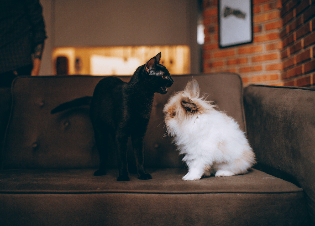
wget -O assets/catdog.jpg https://assets.digitalocean.com/articles/visualize_neural_network/step2b.jpg

Finally, run the pretrained image classifier on the newly downloaded image:

python step_2_pretrained.py assets/catdog.jpg

This will produce the following output, showing your animal classifier works as expected:

Output
Prediction: Persian cat

That concludes running inference with your pretrained model.

Although this neural network produces predictions correctly, we don’t understand how the model arrived at its prediction. To better understand this, start by considering the cat and dog image that you provided to the image classifier.

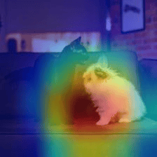
The image classifier predicts Persian cat. One question you can ask is: Was the model looking at the cat on the left? Or the dog on the right? Which pixels did the model use to make that prediction? Fortunately, we have a visualization that answers this exact question. Following is a visualization that highlights pixels that the model used, to determine Persian Cat.

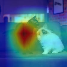
The model classifies the image as Persian cat by looking at the cat. For this tutorial, we will refer to visualizations like this example as saliency maps, which we define to be heatmaps that highlight pixels influencing the final prediction. There are two types of saliency maps:

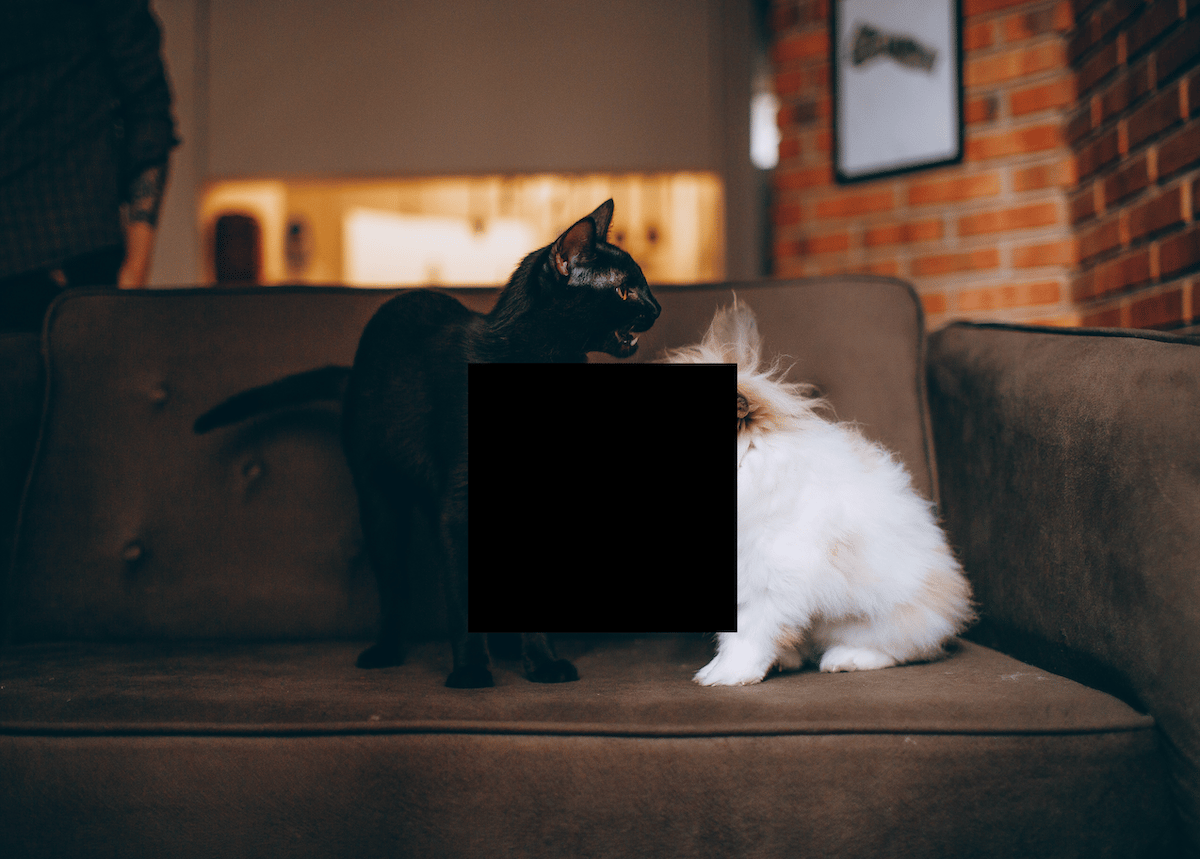
1. Model-agnostic Saliency Maps (often called “black-box” methods): These approaches do not need access to the model weights. In general, these methods change the image and observe the changed image’s impact on accuracy. For example, you might remove the center of the image (pictured following). The intuition is: If the image classifier now misclassifies the image, the image center must have been important. We can repeat this and randomly remove parts of the image each time. In this way, we can produce a heatmap like previously, by highlighting the patches that damaged accuracy the most.

2. Model-aware Saliency Maps (often called “white-box” methods): These approaches require access to the model’s weights. We will discuss one such method in more detail in the next section.

This concludes our brief overview of saliency maps. In the next step, you will implement one model-aware technique called a Class Activation Map (CAM).

Step 3 — Generating Class Activation Maps (CAM)

Class Activation Maps (CAMs) are a type of model-aware saliency method. To understand how a CAM is computed, we first need to discuss what the last few layers in a classification network do. Following is an illustration of a typical image-classification neural network, for the method in this paper on Learning Deep Features for Discriminative Localization.

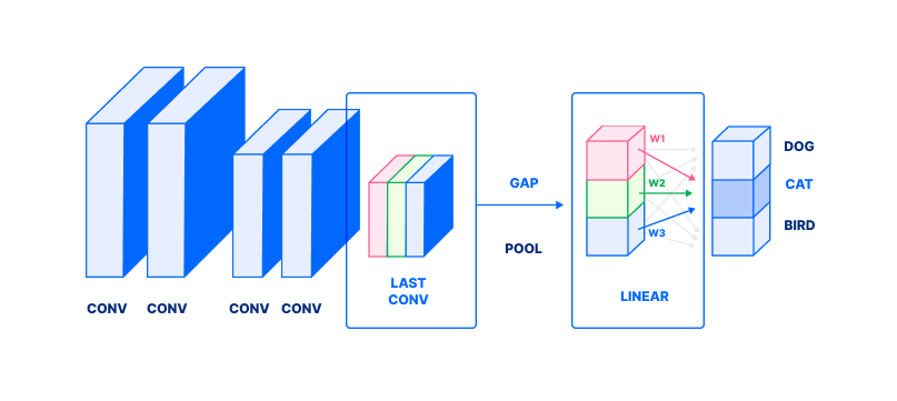
The figure describes the following process in a classification neural network. Note the image is represented as a stack of rectangles; for a refresher on how images are represented as a tensor, see How to Build an Emotion-Based Dog Filter in Python 3 (Step 4):

1. Focus on the second-to-last layer’s outputs, labeled LAST CONV with blue, red, and green rectangles.
2. This output undergoes a global average pool (denoted as GAP). GAP averages values in each channel (colored rectangle) to produce a single value (corresponding colored box, in LINEAR).
3. Finally, those values are combined in a weighted sum (with weights denoted by w1, w2, w3) to produce a probability (dark gray box) of a class. In this case, these weights correspond to CAT. In essence, each wi answers: “How important is the ith channel to detecting a Cat?”
4. Repeat for all classes (light gray circles) to obtain probabilities for all classes.

We’ve omitted several details that are not necessary to explain CAM. Now, we can use this to compute CAM. Let us revisit an expanded version of this figure, still for the method in the same paper. Focus on the second row.

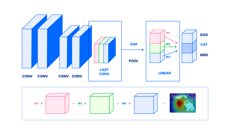
1. To compute a class activation map, take the second-to-last layer’s outputs. This is depicted in the second row, outlined by blue, red, and green rectangles corresponding to the same colored rectangles in the first row.
2. Pick a class. In this case, we pick “Australian Terrier”. Find the weights w1, w2 … wn corresponding to that class.
3. Each channel (colored rectangle) is then weighted by w1, w2 … wn. Note we do not perform a global average pool (step 2 from the previous figure). Compute the weighted sum, to obtain a class activation map (far right, second row in figure).

This final weighted sum is the class activation map.

Next, we will implement class activation maps. This section will be broken into the three steps that we’ve already discussed:

1. Take the second-to-last layer’s outputs.
2. Find weights w1, w2 … wn.
3. Compute a weighted sum of outputs.

Start by creating a new file step_3_cam.py:

nano step_3_cam.py

First, add the Python boilerplate; import the necessary packages and declare a main function:

"""Generate Class Activation Maps"""
import numpy as np
import sys
import torch
import torchvision.models as models
import torchvision.transforms as transforms
import matplotlib.cm as cm

from PIL import Image
from step_2_pretrained import load_image


def main():
    pass


if __name__ == '__main__':
    main()

Create an image loader that will load, resize, and crop your image, but leave the color untouched. This ensures your image has the correct dimensions. Add this before your main function:

. . .
def load_raw_image():
    """Load raw 224x224 center crop of image"""
    image = Image.open(sys.argv[1])
    transform = transforms.Compose([
      transforms.Resize(224),  # resize smaller side of image to 224
      transforms.CenterCrop(224),  # take center 224x224 crop
    ])
    return transform(image)
. . .

In load_raw_image, you first access the one argument passed to the script sys.argv[1]. Then, open the image specified using Image.open. Next, you define a number of different transformations to apply to the images that are passed to your neural network:

• transforms.Resize(224): Resizes the smaller side of the image to 224. For example, if your image is 448 x 672, this operation would downsample the image to 224 x 336.
• transforms.CenterCrop(224): Takes a crop from the center of the image, of size 224 x 224.
• transform(image): Applies the sequence of image transformations defined in the previous lines.

This concludes image loading.

Next, load the pretrained model. Add this function after your first load_raw_image function, but before the main function:

. . .
def get_model():
    """Get model, set forward hook to save second-to-last layer's output"""
    net = models.resnet18(pretrained=True).eval()
    layer = net.layer4[1].conv2

    def store_feature_map(self, _, output):
        self._parameters['out'] = output
    layer.register_forward_hook(store_feature_map)

    return net, layer
. . .

In the get_model function, you:

1. Instantiate a pretrained model models.resnet18(pretrained=True).
2. Change the model’s inference mode to eval by calling .eval().
3. Define layer..., the second-to-last layer, which we will use later.
4. Add a “forward hook” function. This function will save the layer’s output when the layer is executed. We do this in two steps, first defining a store_feature_map hook and then binding the hook with register_forward_hook.
5. Return both the network and the second-to-last layer.

This concludes model loading.

Next, compute the class activation map itself. Add this function before your main function:

. . .
def compute_cam(net, layer, pred):
    """Compute class activation maps

    :param net: network that ran inference
    :param layer: layer to compute cam on
    :param int pred: prediction to compute cam for
    """

    # 1. get second-to-last-layer output
    features = layer._parameters['out'][0]

    # 2. get weights w_1, w_2, ... w_n
    weights = net.fc._parameters['weight'][pred]

    # 3. compute weighted sum of output
    cam = (features.T * weights).sum(2)

    # normalize cam
    cam -= cam.min()
    cam /= cam.max()
    cam = cam.detach().numpy()
    return cam
. . .

The compute_cam function mirrors the three steps outlined at the start of this section and in the section before.

1. Take the second-to-last layer’s outputs, using the feature maps our forward hook saved in layer._parameters.
2. Find weights w1, w2 … wn in the final linear layer net.fc_parameters['weight']. Access the predth row of weights, to obtain weights for our predicted class.
3. Compute a weighted sum of outputs. (features.T * weights).sum(...). The argument 2 means we compute a sum along the index 2 dimension of the provided tensor.
4. Normalize the class activation map, so that all values fall in between 0 and 1—cam -= cam.min(); cam /= cam.max().
5. Detach the PyTorch tensor from the computation graph .detach(). Convert the CAM from a PyTorch tensor object into a numpy array. .numpy().

This concludes computation for a class activation map.

Our last helper function is a utility that saves the class activation map. Add this function before your main function:

. . .
def save_cam(cam):
    # save heatmap
    heatmap = (cm.jet_r(cam) * 255.0)[..., 2::-1].astype(np.uint8)
    heatmap = Image.fromarray(heatmap).resize((224, 224))
    heatmap.save('heatmap.jpg')
    print(' * Wrote heatmap to heatmap.jpg')

    # save heatmap on image
    image = load_raw_image()
    combined = (np.array(image) * 0.5 + np.array(heatmap) * 0.5).astype(np.uint8)
    Image.fromarray(combined).save('combined.jpg')
    print(' * Wrote heatmap on image to combined.jpg')
. . .

This utility save_cam performs the following:

1. Colorize the heatmap cm.jet_r(cam). The output is in the range [0, 1] so multiply by 255.0. Furthermore, the output (1) contains a 4th alpha channel and (2) the color channels are ordered as BGR. We use indexing [..., 2::-1] to solve both problems, dropping the alpha channel and inverting the color channel order to be RGB. Finally, cast to unsigned integers.
2. Convert the image Image.fromarray into a PIL image and use the image’s image-resize utility .resize(...), then the .save(...) utility.
3. Load a raw image, using the utility load_raw_image we wrote earlier.
4. Superimpose the heatmap on top of the image by adding 0.5 weight of each. Like before, cast the result to unsigned integers .astype(...).
5. Finally, convert the image into PIL, and save.

Next, populate the main function with some code to run the neural network on a provided image:

. . .
def main():
    """Generate CAM for network's predicted class"""
    x = load_image()
    net, layer = get_model()

    out = net(x)
    _, (pred,) = torch.max(out, 1)  # get class with highest probability

    cam = compute_cam(net, layer, pred)
    save_cam(cam)
. . .

In main, run the network to obtain a prediction.

1. Load the image.
2. Fetch the pretrained neural network.
3. Run the neural network on the image.
4. Find the highest probability with torch.max. pred is now a number with the index of the most likely class.
5. Compute the CAM using compute_cam.
6. Finally, save the CAM using save_cam.

This now concludes our class activation script. Save and close your file. Check that your script matches the step_3_cam.py in this repository.

Then, run the script:

python step_3_cam.py assets/catdog.jpg

Your script will output the following:

Output
 * Wrote heatmap to heatmap.jpg
 * Wrote heatmap on image to combined.jpg

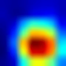
This will produce a heatmap.jpg and combined.jpg akin to the following images showing the heatmap and the heatmap combined with the cat/dog image.

You have produced your first saliency map. We will end the article with more links and resources for generating other kinds of saliency maps. In the meantime, let us now explore a second approach to explainability—namely, making the model itself interpretable.

Step 4 — Using Neural-Backed Decision Trees

Decision Trees belong to a family of rule-based models. A decision tree is a data tree that displays possible decision pathways. Each prediction is the result of a series of predictions.

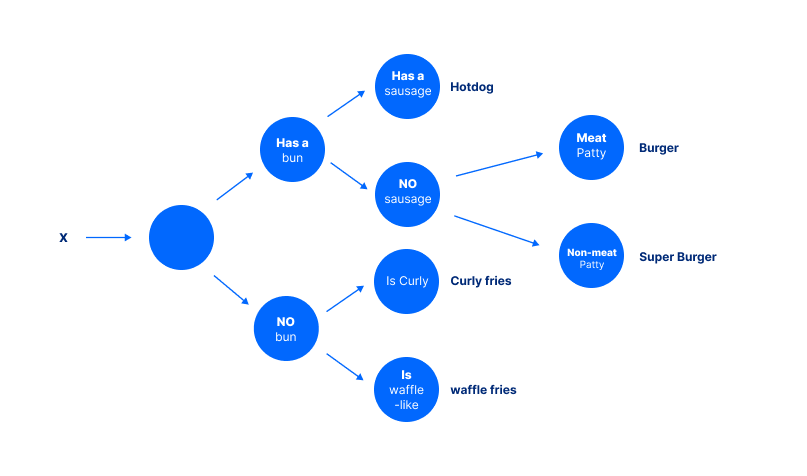
Instead of just outputting a prediction, each prediction also comes with justification. For example, to arrive at the conclusion of “Hotdog” for this figure the model must first ask: “Does it have a bun?”, then ask: “Does it have a sausage?” Each of these intermediate decisions can be verified or challenged separately. As a result, classic machine learning calls these rule-based systems “interpretable.”

One question is: How are these rules created? Decision Trees warrant a far more detailed discussion of its own but in short, rules are created to “split classes as much as possible.” Formally, this is “maximizing information gain.” In the limit, maximizing this split makes sense: If the rules perfectly split classes, then our final predictions will always be correct.

Now, we move on to using a neural network and decision tree hybrid. For more on decision trees, see Classification and Regression Trees (CART) overview.

Now, we will run inference on a neural network and decision tree hybrid. As we will find, this gives us a different type of explainability: direct-model interpretability.

Start by creating a new file called step_4_nbdt.py:

nano step_4_nbdt.py

First, add the Python boilerplate. Import the necessary packages and declare a main function. maybe_install_wordnet sets up a prerequisite that our program may need:

"""Run evaluation on a single image, using an NBDT"""

from nbdt.model import SoftNBDT, HardNBDT
from pytorchcv.models.wrn_cifar import wrn28_10_cifar10
from torchvision import transforms
from nbdt.utils import DATASET_TO_CLASSES, load_image_from_path, maybe_install_wordnet
import sys

maybe_install_wordnet()


def main():
    pass


if __name__ == '__main__':
    main()

Start by loading the pretrained model, as before. Add the following before your main function:

. . .
def get_model():
    """Load pretrained NBDT"""
    model = wrn28_10_cifar10()
    model = HardNBDT(
      pretrained=True,
      dataset='CIFAR10',
      arch='wrn28_10_cifar10',
      model=model)
    return model
. . .

This function does the following:

1. Creates a new model called WideResNet wrn28_10_cifar10().
2. Next, it creates the neural-backed decision tree variant of that model, by wrapping it with HardNBDT(..., model=model).

This concludes model loading.

Next, load and preprocess the image for model inference. Add the following before your main function:

. . .
def load_image():
    """Load + transform image"""
    assert len(sys.argv) > 1, "Need to pass image URL or image path as argument"
    im = load_image_from_path(sys.argv[1])
    transform = transforms.Compose([
      transforms.Resize(32),
      transforms.CenterCrop(32),
      transforms.ToTensor(),
      transforms.Normalize((0.4914, 0.4822, 0.4465), (0.2023, 0.1994, 0.2010)),
    ])
    x = transform(im)[None]
    return x
. . .

In load_image, you start by loading the image from the provided URL, using a custom utility method called load_image_from_path. Next, you define a number of different transformations to apply to the images that are passed to your neural network:

• transforms.Resize(32): Resizes the smaller side of the image to 32. For example, if your image is 448 x 672, this operation would downsample the image to 32 x 48.
• transforms.CenterCrop(224): Takes a crop from the center of the image, of size 32 x 32.
• transforms.ToTensor(): Converts the image into a PyTorch tensor. All PyTorch models require PyTorch tensors as input.
• transforms.Normalize(mean=..., std=...): Standardizes your input by subtracting the mean, then dividing by the standard deviation. This is described more precisely in the torchvision documentation.

Finally, apply the image transformations to the image transform(im)[None].

Next, define a utility function to log both the prediction and the intermediate decisions that led up to it. Place this before your main function:

. . .
def print_explanation(outputs, decisions):
    """Print the prediction and decisions"""
    _, predicted = outputs.max(1)
    cls = DATASET_TO_CLASSES['CIFAR10'][predicted[0]]
    print('Prediction:', cls, '// Decisions:', ', '.join([
        '{} ({:.2f}%)'.format(info['name'], info['prob'] * 100) for info in decisions[0]
    ][1:]))  # [1:] to skip the root
. . .

The print_explanations function computes and logs predictions and decisions:

1. Starts by computing the index of the highest probability class outputs.max(1).
2. Then, it converts that prediction into a human readable class name using the dictionary DATASET_TO_CLASSES['CIFAR10'][predicted[0]].
3. Finally, it prints the prediction cls and the decisions info['name'], info['prob']....

Conclude the script by populating the main with utilities we have written so far:

. . .
def main():
    model = get_model()
    x = load_image()
    outputs, decisions = model.forward_with_decisions(x)  # use `model(x)` to obtain just logits
    print_explanation(outputs, decisions)

We perform model inference with explanations in several steps:

1. Load the model get_model.
2. Load the image load_image.
3. Run model inference model.forward_with_decisions.
4. Finally, print the prediction and explanations print_explanations.

Close your file, and double-check your file contents matches step_4_nbdt.py. Then, run your script on the photo from earlier of two pets side-by-side.

python step_4_nbdt.py assets/catdog.jpg

This will output the following, both the prediction and the corresponding justifications.

Output
Prediction: cat // Decisions: animal (99.34%), chordate (92.79%), carnivore (99.15%), cat (99.53%)

This concludes the neural-backed decision tree section.

Conclusion

You have now run two types of Explainable AI approaches: a post-hoc explanation like saliency maps and a modified interpretable model using a rule-based system.

There are many explainability techniques not covered in this tutorial. For further reading, please be sure to check out other ways to visualize and interpret neural networks; the utilities number many, from debugging to debiasing to avoiding catastrophic errors. There are many applications for Explainable AI (XAI), from sensitive applications like medicine to other mission-critical systems in self-driving cars.

• Other model-aware saliency methods: Grad-CAM: Visual Explanations from Deep Networks via Gradient-based Localization paper, Grad-CAM++: Improved Visual Explanations for Deep Convolutional Networks, and this code in the Grad-CAM implementation in Pytorch repository.
• Model-agnostic saliency methods: RISE, LIME, and LIME implementation in PyTorch repository.
• Interpretable models via neural network and decision tree hybrids: Neural-Backed Decision Trees, Deep Neural Decision Tree, Neural-Backed Decision Trees implementation in PyTorch repository.
• There are also other forms of explainability not discussed, such as Feature Visualization via Distill and Influence Analysis.