AI Technical Writer

Introduction
When dealing with data where the outcome is qualitative, such as predicting whether a customer will make a purchase or whether an employee will remain in an organization, the results cannot be directly measured on a numerical scale. These types of outcomes are categorical in nature and typically take the form of binary choices (yes/no, 1/0). To analyze such situations, economists and data scientists often rely on models designed for binary outcomes, one of the most straightforward being the Linear Probability Model (LPM).
Now, there might be a question of why economists are worried about linear probability model (LPM)?
Economists often use these models because much of their research deals with choices and decisions that are naturally binary.
For example:
- Does a household buy insurance or not?
- Does a worker participate in the labor force or not?
- Does a loan applicant default or repay?
While data scientists often focus on the prediction part (e.g., will this user click an ad), economists care about the interpretation, theory testing, and causal insights. They want to understand why people make these choices, not just whether they will.
The Linear Probability Model (LPM) gives economists a simple way to link binary outcomes with explanatory variables like income, education, or policy changes. The LPM provides a straightforward way to link these binary choices with explanatory factors such as income, education, or policy changes. Even if it’s not the most accurate model, it remains valuable for building intuition and testing economic theories.
That’s why, historically, economists leaned on LPM as a starting point and then moved toward more refined models like logit and probit for better accuracy.
In this article, we will understand LPM in detail, the key benefits that make it simple and intuitive, the important drawbacks that limit its reliability, and practical examples of how to implement it in Python. We’ll also look at how it compares with alternatives like logit and probit models, so you’ll know when an LPM makes sense and when it’s better to use something more advanced.
Key Takeaways
- The Linear Probability Model (LPM) is a simple way to estimate probabilities for binary outcomes using ordinary least squares (OLS).
- It is easy to understand and interpret, which is why economists and data analysts still use it as a starting point.
- However, LPM has serious drawbacks such as predictions outside the [0,1] range, heteroskedasticity, and non-normal errors that can make results misleading if not handled carefully.
- Despite these issues, LPM can provide quick insights and serve as a benchmark model before moving to more sophisticated methods.
Prerequisites
- Linear Regression – Understanding how the regression model works. LPM is essentially applying these ideas to a binary dependent variable.
- Ordinary Least Squares (OLS) – The method used to estimate regression coefficients by minimizing the sum of squared errors. Since LPM relies on OLS, knowing how OLS works is essential.
- Logistic Regression (Logit Model) – The most common alternative to LPM, where probabilities are modeled with the logistic function. Having a basic idea of how logistic regression works makes it easier to compare.
- Probability & Bernoulli Trials – Since the dependent variable in LPM is binary (0/1), knowing the basics of probability distributions and Bernoulli random variables will help interpret results.
What is the Linear Probability Model?
The Linear Probability Model (LPM) is one of the simplest methods to model the outcome of the dependent variable that is binary in nature. Here, the dependent variable can take the value yes (1) or no (0).
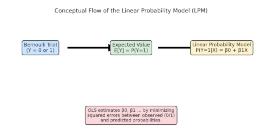
We can think of each observation as a Bernoulli trial:
- A Bernoulli trial is a random experiment with only two outcomes (success = 1, failure = 0).
- For example, flipping a coin and recording heads as 1 and tails as 0 is a Bernoulli trial.
- The key idea is that the expected value of a Bernoulli random variable equals its probability of success.
The LPM takes this idea and connects the probability of success (pi) to explanatory variables X using a linear equation:
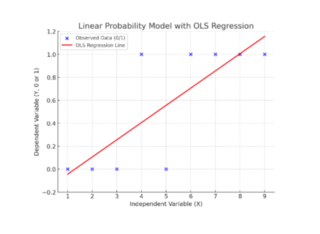
Here is where the concept of Ordinary Least Squares (OLS) comes in:
OLS is the standard estimation method for linear regression. It works by finding the line (or hyperplane in multiple dimensions) that minimizes the sum of squared differences between the actual values of Yi (0 or 1) and the predicted values (Ŷ). Even though Yi is binary, OLS can still be applied. The regression coefficients (β) show how changes in the independent variables affect the probability of Yi=1.
Mathematical Definition of LPM
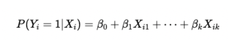
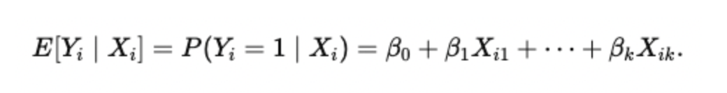
As we understood, the LPM links a binary dependent variable to one or more explanatory variables using a linear regression framework. The equation is represented by the following mathematical expression:
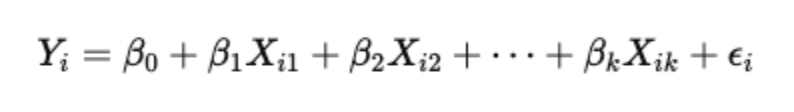
Where:
- Yi: Binary dependent variable (1 if the outcome is present, 0 if not).
- β0: Intercept, representing the baseline probability when all predictors are zero.
- βk: Coefficients, which measure how a one-unit change in Xk affects the probability of Y=1.
- Xik: Explanatory (independent) variables.
- ϵi: Error term, capturing the difference between the predicted probability and the actual observed outcome.
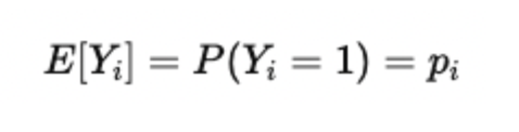
Because Yi is binary (a random variable), its expected value is equal to the probability of success:

Substituting this in the equation gives:
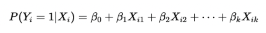
This means the predicted value from the regression (Ŷ) is directly interpreted as the probability that the outcome occurs.
Why is it called a “Probability Model”?
It is called a probability model because the predicted values of the dependent variable are interpreted as probabilities. For example:
- If the model predicts Ŷi = 0.75, this means there is a 75% probability that the outcome will occur.
- Similarly, Ŷi = 0.20 implies only a 20% chance of occurrence.
Unlike ordinary regression, where predicted values represent continuous outcomes (e.g., test scores, prices), in the LPM, they represent probabilities of binary events. Let us take a numerical example to understand the concept better:
Suppose an economist is studying the probability that a loan applicant defaults on a loan (Y=1) based on two factors: income and credit score.
If we include this in our estimated LPM equation, it might look like this:
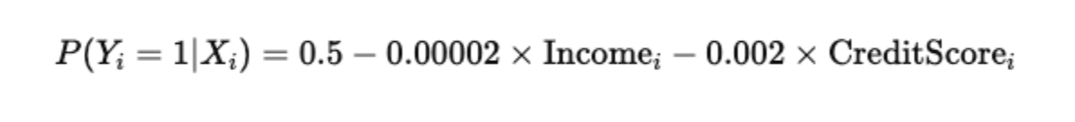
Interpretation of coefficients:
- Intercept (0.5): If both income and credit score were zero (a hypothetical baseline), the model predicts a 50% chance of default.
- Income coefficient (-0.00002): For every additional dollar of income, the probability of default decreases by 0.002 percentage points.
- Credit Score coefficient (-0.002): For every one-point increase in credit score, the probability of default decreases by 0.2 percentage points.
Now, consider an applicant with:
- Income = $40,000
- Credit Score = 650
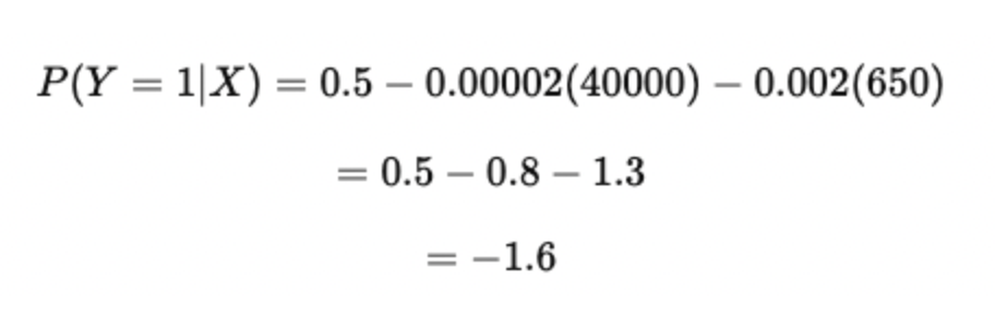
This calculation highlights a well-known limitation of the LPM that the model can produce probabilities less than 0 (or greater than 1), which are not meaningful. We will discuss more of these limitations and how to tackle in later part of the article.
Still, the interpretation of the coefficients (how income and credit score affect default risk) can provide valuable insights, even if the predicted probability itself is invalid.
Assumptions and Properties
Certain assumptions must be made when dealing with the LPM model. Let us discuss each one of them in detail.
- Linearity in parameters: This condition expects Y, the dependent variable, to be a linear function of the predictors:
OLS estimates the best linear predictor (in the least-squares sense). If the true conditional probability is highly nonlinear in X, LPM will give the best linear approximation but may miss important curvature.
- Random sampling / independent observations: Observations are independent of each other to remove bias.
- No multicollinearity: The independent variables should not be correlated with each other, as this may again lead to bias. Drop or combine collinear variables, or use dimensionality reduction. This assumption ensures that coefficients can be uniquely estimated.
- Normal Distribution of Errors: For valid hypothesis testing, OLS assumes normally distributed errors. In LPM, the dependent variable is binary (0/1), so the error term is also binary, not continuous or normally distributed. This makes exact inference problematic, though large-sample properties (via the Central Limit Theorem) often help.
Hands-on Example: Implementing LPM
We’ll use study hours and attendance rate as predictors to model whether a student passes an exam (1) or fails (0).
import pandas as pd
import numpy as np
import statsmodels.api as sm

# ----------------------------
# Create synthetic dataset
# ----------------------------
np.random.seed(42)
n = 100

# Independent variables
study_hours = np.random.randint(0, 10, n)
attendance = np.random.randint(50, 100, n)  # percentage

# Binary outcome (pass=1, fail=0)
# Rule: more hours + higher attendance = higher probability
prob_pass = 0.2 + 0.08 * study_hours + 0.005 * attendance
prob_pass = np.clip(prob_pass, 0, 1)  # ensure probabilities in [0,1]

exam_result = np.random.binomial(1, prob_pass)

# Build DataFrame
df = pd.DataFrame({
    "study_hours": study_hours,
    "attendance": attendance,
    "exam_result": exam_result
})

# ----------------------------
# Fit Linear Probability Model
# ----------------------------
X = sm.add_constant(df[["study_hours", "attendance"]])  # predictors + intercept
y = df["exam_result"]

lpm = sm.OLS(y, X).fit()

print(lpm.summary())
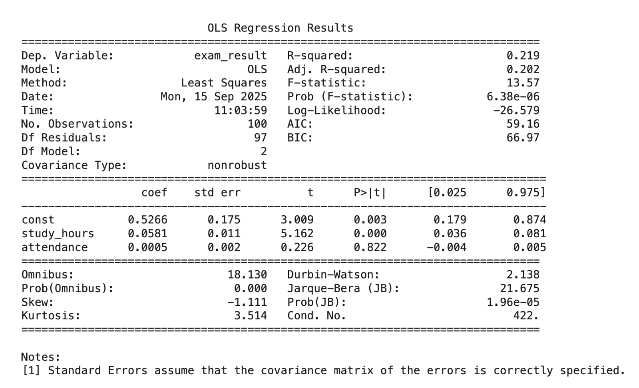
R-squared = 0.219 → About 21.9% of the variation in passing is explained by study hours and attendance. → Not super high (expected, since exam outcomes depend on more factors).
| Variable | Coefficient Interpretation | |
|---|---|---|
| Intercept (const = 0.5266) | When study_hours = 0 and attendance = 0, predicted probability of passing = 52.7%. (Baseline probability.) | |
| study_hours (0.0581, p < 0.001) | Each extra study hour increases the probability of passing by about 5.8 percentage points. This effect is statistically significant. | |
| attendance (0.0005, p = 0.822) | Each 1% increase in attendance increases the probability of passing by only 0.05 percentage points. But the p-value is very high (0.822) → this effect is not statistically significant. |
Statistical Significance
- study_hours: Very strong evidence (p < 0.001) → a real predictor of passing.
- attendance: No evidence (p ≈ 0.82) → likely doesn’t matter in this dataset.
Linear probability model interpretation
- Studying matters a lot: Every hour adds ~6% probability of passing.
- Attendance doesn’t matter here: Maybe because most students already had high attendance (not much variation).
- Intercept (~53%): Even with zero study hours and attendance, students still had ~50% chance (suggests other unobserved factors like prior knowledge, test difficulty).
- Model Limitations: Since this is an LPM, predicted probabilities could go below 0 or above 1 for extreme values.
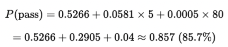
Example Prediction:
For a student with 5 study hours and 80% attendance:
Limitations of the Linear Probability Model
The Linear Probability Model is simple and intuitive, but it has some serious statistical and practical drawbacks that limit its usefulness. Let’s understand them one by one.
1. Non-normality of the error term
In LPM, the dependent variable is binary (0 or 1). This means the error term (ϵ) cannot follow a normal distribution, which is a key assumption of OLS. Instead, the error takes only two values, depending on whether the prediction was correct or not. This breaks the standard assumptions used for hypothesis testing.
However, thanks to the Central Limit Theorem, if the sample size is large enough, the average of these errors tends to approximate a normal distribution. This is why in large datasets, LPM still provides somewhat usable estimates, even though technically the error is not normal.
2. Heteroskedasticity
Heteroskedasticity means the error term does not have constant variance. In the LPM, the variance of the error term depends on the predicted probability, given by:
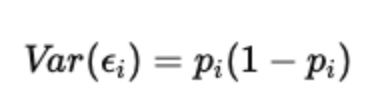
This means that when the predicted probability is near 0.5, the variance is large, and when it’s near 0 or 1, the variance is small. For example, predicting whether someone buys a product: people with ~50% probability contribute more noisy variation than those who are almost certain to buy (p ≈ 1) or not buy (p ≈ 0).
To fix this, we can use Weighted Least Squares (WLS) instead of plain OLS. WLS adjusts the regression by giving less weight to observations with higher variance and more weight to those with lower variance, stabilizing the model.
3. Bounded dependent variable
Probabilities must lie between 0 and 1. Now, because it’s a linear function, it can predict probabilities less than 0 or greater than 1, which makes no sense in practice. For instance, the model might predict a “-0.2” probability that someone buys a car, which is meaningless.
One partial solution is to use Restricted Least Squares, which forces coefficients to generate probabilities only within [0, 1]. However, this makes the model more complex and less natural than using alternatives like logit or probit.
4. Lower R-squared values
The coefficient of determination (R²) in an LPM is often low compared to standard regressions. This happens because a binary outcome has limited variation, and a linear regression struggles to capture it. A low R² does not always mean the model is useless, but it highlights how poorly LPM explains variation compared to logistic regression.
5. Predictions outside [0,1]
As mentioned earlier, because LPM is linear, some predicted values will fall below 0 or above 1. This is not just a theoretical issue, but in real applications, you’ll see predictions like 1.2 or -0.15, which cannot be probabilities. This is one of the strongest reasons why economists often prefer nonlinear models like logit and probit, which naturally restrict predictions to the [0,1] range.
The LPM is easy to understand and compute, but it struggles with statistical assumptions (like non-normality and heteroskedasticity), practical interpretation (probabilities outside [0,1]), and explanatory power (low R² and possible misspecification).
Logit and Probit Models
Because the Linear Probability Model often predicts invalid probabilities (less than 0 or greater than 1) and assumes a straight-line relationship, a well-known alternative to this approach is the logit and probit models.
- Logit Model: Uses the logistic function to map any value of the predictors into a probability between 0 and 1. It assumes the relationship between predictors and the outcome is S-shaped rather than linear. This makes it more realistic for probability data.
- Probit Model: Similar to logit, but instead of the logistic function, it uses the cumulative normal distribution to constrain probabilities between 0 and 1. It’s often chosen when the assumption of normally distributed errors makes sense.
Both of these models solve the biggest problems of LPM by ensuring probabilities stay within [0,1] and by better capturing nonlinear relationships.
Pros of the LPM
While the Linear Probability Model has its limitations, it can still serve as a useful starting point for model building before moving on to more advanced techniques like logit or probit. The model is simple to estimat, and its coefficients are easy to interpret, directly reflecting the change in probability of the outcome variable. Unlike many complex models, LPM is not a “black box,” and it allows for a clear understanding of cause-and-effect relationships, making the results more transparent and explainable.
FAQ’s
Q1. What is the linear probability model used for?
The Linear Probability Model (LPM) is used when you want to study a binary outcome, that is, when the dependent variable can only take two values, usually 0 or 1. For example, whether someone buys a product (1) or not (0), whether a person is employed (1) or unemployed (0), or whether a loan is approved (1) or denied (0). The model applies ordinary least squares (OLS) regression to these binary outcomes. The main appeal of LPM is its simplicity: the coefficients can be interpreted as the change in probability of the outcome occurring when the independent variable changes by one unit.
Q2. Why is the linear probability model problematic?
Even though the LPM is simple, it comes with serious issues. First, it can predict probabilities outside the range of 0 and 1, which doesn’t make sense because probabilities can’t be negative or greater than 1. Second, the error term in LPM is not normally distributed, since the dependent variable is binary, and this breaks one of the key assumptions of OLS regression. Third, the variance of the errors depends on the values of the independent variables, making the model heteroskedastic. This invalidates standard OLS inference unless corrected. Finally, LPM often has lower explanatory power (low R²) compared to non-linear models. These problems mean that while it’s useful as a teaching tool or first step, it’s not always the best tool for final analysis.
Q3. What are the alternatives to the LPM?
The most common alternatives are logit and probit models. Both of these are nonlinear regression models specifically designed for binary outcomes. Instead of fitting a straight line, they map the predicted probabilities onto a curve that is naturally bounded between 0 and 1. This ensures predictions are always valid probabilities. Logit models use the logistic function, while probit models use the cumulative distribution function of a standard normal distribution. These models handle the limitations of LPM much better, especially when you want reliable probability estimates or when heteroskedasticity is a concern.
Q4. How do I implement an LPM in Python?
Implementing an LPM in Python is straightforward. You can use the statsmodels or scikit-learn libraries. For example, with statsmodels, you can run an ordinary least squares (OLS) regression with a binary dependent variable:
import statsmodels.api as sm

# Example dataset
X = df[['age', 'income']]  # independent variables
y = df['buy']              # dependent binary variable (0/1)

# Add a constant for intercept
X = sm.add_constant(X)

# Fit the linear probability model using OLS
model = sm.OLS(y, X).fit()

print(model.summary())
The results will show you the coefficients, which you can interpret as the change in probability of the outcome (e.g., buying the product) given a one-unit change in the predictor.
Q5. When is it acceptable to use the linear probability model?
The LPM is most acceptable in situations where simplicity and interpretability matter more than perfect prediction. For example, if your goal is to get a quick, rough idea of how different factors affect the probability of an outcome, LPM works well. It’s also often used in teaching econometrics to illustrate key concepts. Some applied researchers still use it when the dataset is large and the main purpose is to estimate marginal effects rather than precise probability predictions. However, if your focus is on accurate prediction, valid standard errors, or probabilities strictly within [0,1], then switching to a logit or probit model is the better choice.
Conclusion
The Linear Probability Model (LPM) is one of the simplest ways to model binary outcomes using regression. The biggest strength lies in its simplicity and ease of interpretation, where the coefficients can directly tell how the changes in predictors affect the probability of an event.
However, its simplicity comes with trade-offs, including unrealistic predictions outside the [0,1] range, heteroskedastic errors, and lower accuracy compared to more advanced models. In practice, researchers often start with an LPM to gain initial insights and then move toward logit or probit models for more reliable results. The key is to understand the model’s strengths and weaknesses so you know when it can serve your purpose and when it’s time to move on to alternatives.
Thanks for learning with the DigitalOcean Community. Check out our offerings for compute, storage, networking, and managed databases.
About the author
With a strong background in data science and over six years of experience, I am passionate about creating in-depth content on technologies. Currently focused on AI, machine learning, and GPU computing, working on topics ranging from deep learning frameworks to optimizing GPU-based workloads.
Still looking for an answer?
This textbox defaults to using Markdown to format your answer.
You can type !ref in this text area to quickly search our full set of tutorials, documentation & marketplace offerings and insert the link!
 This work is licensed under a Creative Commons Attribution-NonCommercial- ShareAlike 4.0 International License.
Become a contributor for community
Get paid to write technical tutorials and select a tech-focused charity to receive a matching donation.

DigitalOcean Documentation
Full documentation for every DigitalOcean product.

Resources for startups and AI-native businesses
The Wave has everything you need to know about building a business, from raising funding to marketing your product.
The developer cloud
Scale up as you grow — whether you're running one virtual machine or ten thousand.

Start building today
From GPU-powered inference and Kubernetes to managed databases and storage, get everything you need to build, scale, and deploy intelligent applications.
