ReLU vs ELU: Picking the Right Activation for Deep Nets

Activation functions are one of the key factors behind the success of deep learning. They are non‑linear transforms that give artificial neural networks the power to model complex relationships. Without them, each layer would multiply inputs by weights and add biases, resulting in a linear regression. The Non‑linearities allow the network to learn more complex patterns and enable deep architectures. ReLU and ELU are two of the most popular and widely discussed activation functions. They are both proposed as solutions to the vanishing gradient problem.

In this article, we will cover the internal workings of ReLU (Rectified Linear Unit) and ELU (Exponential Linear Unit), their strengths and weaknesses compared to each other, demonstrate their implementation in major frameworks, and provide some guidelines for when to use each.

• ReLU = speed & simplicity; ELU = stability. ReLU is the fastest robust default; ELU incurs a small constant-factor compute cost for more stable and faster optimization with no dead units.
• Gradient behavior matters. ReLU zeros out negatives (can lead to dead neurons), whereas ELU has a non-zero negative slope, and also pushes activations towards zero mean.
• BatchNorm narrows the gap. With proper He/Kaiming init and BatchNorm, ReLU often matches ELU in final accuracy.
• Context is key. Use ReLU/Leaky ReLU for latency/edge and quantization; experiment with ELU when training is unstable or zero-centering activations seems helpful.

• Math & ML basics: Comfortable with linear algebra (vectors/matrices), calculus (derivatives), and the training loop (forward/backprop, loss, gradients). Know what vanishing gradients, initialization (He/Kaiming), and BatchNorm are.
• Python + tooling: Working Python 3.9+ with NumPy and matplotlib; able to run notebooks or scripts.
• Deep-learning frameworks: Basic familiarity with TensorFlow/Keras (layers, models, compile/fit/evaluate). PyTorch experience is a plus.

A neural network accepts an input vector and performs a weighted sum (dot product) on the input and adds biases to the result. The output is then executed through an activation function, which determines whether a neuron should “fire” and injects non‑linearity into the model. Without non‑linear activation functions, multiple linear layers stacked on top of each other would result in a single linear transformation. Sigmoid and tanh activation functions were used in early neural networks. However, they are susceptible to vanishing gradient problems, as gradients become infinitesimally small in saturating regions, leading to very slow learning in earlier layers of the network. As a result, rectifier functions were introduced to address this issue.

The Rectified Linear Unit is probably the most commonly used activation function in modern deep learning. It’s a piecewise linear function that can be defined as below:

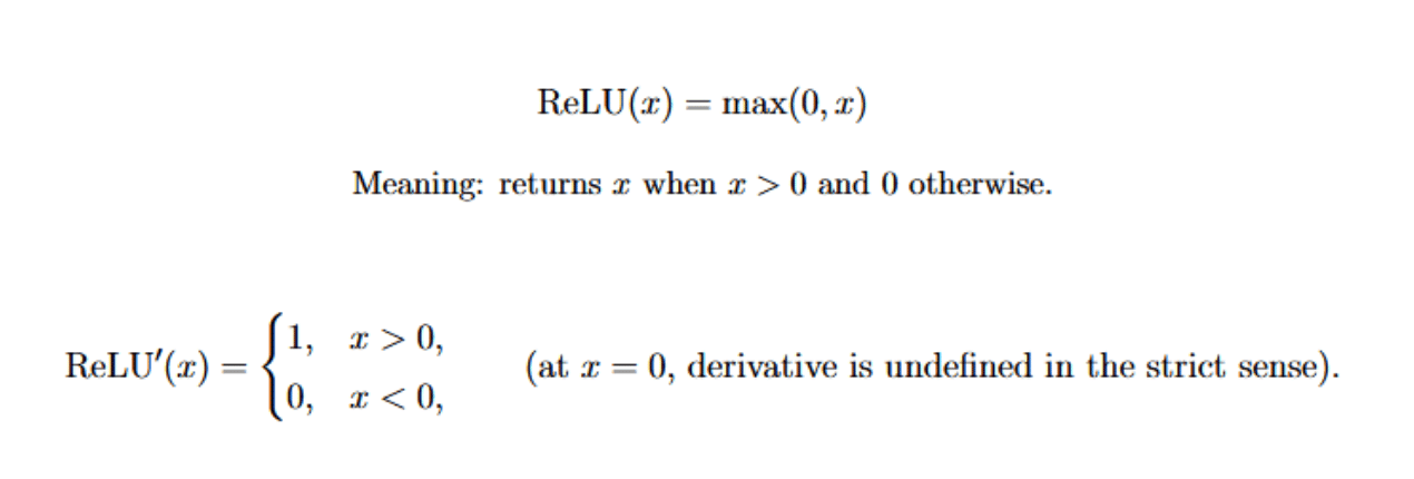
Gradients therefore flow unchanged for positive inputs, but are zero for non‑positive inputs.

Benefits of ReLU

• The vanishing gradient problem is mitigated. Since the derivative of ReLU is always 1 for positive numbers, the gradient will not vanish as it backpropagates through layers.
• Computationally inexpensive. It involves only a comparison operation, so the hardware implementation is efficient. This makes it a faster operation than functions requiring exponentials or divisions.
• Sparse activation. For negative inputs, the output of ReLU is zero. This means that the majority of the neurons will be inactive for a given input, resulting in sparse activation. This leads to faster and efficient computation and can act as an implicit regularizer that improves generalization.
• Simple to implement. ReLU has a very simple formula that is easy to implement in any deep‑learning framework.

Drawbacks of ReLU

• Dying ReLU problem. If the input to a neuron is negative, then the derivative is zero. This prevents the neuron from updating its weights during training. Once this state has been reached, the neuron may never fire again, creating a “dead” neuron.
• Unbounded positive output. The ReLU’s output range is [0,∞). This can lead to large positive activations, which can cause the weight updates to explode, particularly if learning rates are not carefully tuned.
• Non‑differentiability at zero. The derivative is undefined at exactly 0. In practice, most frameworks either define a subgradient or otherwise deal with the point smoothly.

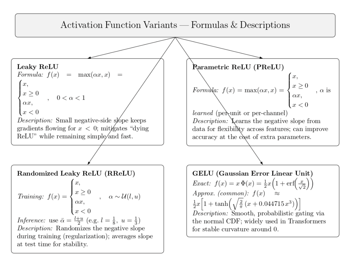
Variants of ReLU

A few variants of ReLU have been proposed to address its shortcomings. While these alleviate some issues, the vanilla RELU remains the default choice because of its simplicity.

The Exponential Linear Unit was proposed by Clevert, Unterthiner, and Hochreiter in 2015. ELU, similar to ReLU, returns the identity for positive inputs. For negative inputs, it has an exponential form controlled by a parameter α:

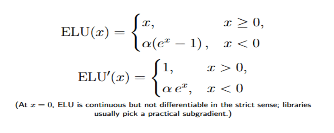
Note that in practice, α is often set to 1. In this case, it produces a smooth negative output that asymptotically approaches −α as x→−∞. The function is continuous and everywhere differentiable (apart from possibly at zero, when α≠1).

Benefits of ELU

• Faster learning and better generalization: The original ELU paper reports that networks trained with ELUs learn faster and generalize better than those trained with ReLUs or Leaky ReLUs.
• Shifts activations closer to zero: The ELU provides negative outputs for negative inputs, which brings the activations closer to zero and mitigates the bias shift effect (scenarios where non‑zero mean activations provide a bias term for the next layer). Zero‑centered activations also enable the standard gradient to better approximate the natural gradient, which can speed learning.
• Noise‑robust deactivation: The ELU saturates to a negative value for large negative inputs, providing a noise‑robust deactivation state. This property reduces variation when neurons are deactivated.
• No dying neuron problem: The ELU has a non‑zero gradient for negative inputs, so neurons can continue to learn when receiving negative signals (a problem that occurs for ReLU).

The script below is a short, reproducible benchmark. It plots popular activations (ReLU, ELU, Leaky ReLU, GELU, Sigmoid). Then it builds the same MLP with the selected activation, trains ReLU and ELU variants of the MLP on MNIST with identical hyperparameters, and prints a direct accuracy comparison on a test set. A small helper also draws validation-accuracy curves to compare convergence across epochs.

import os
import math
import numpy as np
import matplotlib.pyplot as plt
import tensorflow as tf
from tensorflow import keras
from tensorflow.keras import layers

# -------------- Repro --------------
SEED = 1337
tf.keras.utils.set_random_seed(SEED)
np.random.seed(SEED)
os.environ["TF_DETERMINISTIC_OPS"] = "1"

# -------------- Plotting utility --------------
def plot_activations(xmin=-5, xmax=5, points=1000, alpha=1.0, neg_slope=0.01):
    """Visualize common activation functions."""
    x = np.linspace(xmin, xmax, points)

    relu    = np.maximum(0, x)
    elu     = np.where(x >= 0, x, alpha * (np.exp(x) - 1.0))
    lrelu   = np.where(x >= 0, x, neg_slope * x)
    gelu    = 0.5 * x * (1.0 + np.vectorize(math.erf)(x / math.sqrt(2.0)))
    sigmoid = 1.0 / (1.0 + np.exp(-x))

    plt.figure(figsize=(8, 5))
    plt.plot(x, relu,    label="ReLU")
    plt.plot(x, elu,     label=f"ELU (α={alpha})")
    plt.plot(x, lrelu,   label=f"Leaky ReLU ({neg_slope})")
    plt.plot(x, gelu,    label="GELU")
    plt.plot(x, sigmoid, label="Sigmoid")
    plt.title("Common Activation Functions")
    plt.xlabel("x")
    plt.ylabel("activation(x)")
    plt.legend()
    plt.grid(True, alpha=0.3)
    plt.tight_layout()
    plt.show()

# -------------- Model builder --------------
def build_mlp(act="relu", alpha=1.0, input_shape=(784,), num_classes=10, hidden=256, bn=True):
    """Create a simple MLP with a selectable activation."""
    inputs = keras.Input(shape=input_shape)
    x = layers.Dense(hidden, use_bias=not bn)(inputs)
    if bn:
        x = layers.BatchNormalization()(x)

    if act == "relu":
        x = layers.ReLU()(x)
    elif act == "elu":
        x = layers.ELU(alpha=alpha)(x)
    elif act == "leaky_relu":
        x = layers.LeakyReLU(alpha=0.01)(x)
    elif act == "gelu":
        x = layers.Activation(tf.keras.activations.gelu)(x)
    else:
        raise ValueError(f"Unknown activation: {act}")

    outputs = layers.Dense(num_classes)(x)
    model = keras.Model(inputs, outputs, name=f"mlp_{act}")
    return model

# -------------- Data (MNIST) --------------
def load_mnist(flatten=True):
    (x_train, y_train), (x_test, y_test) = keras.datasets.mnist.load_data()
    x_train = x_train.astype("float32") / 255.0
    x_test  = x_test.astype("float32") / 255.0
    if flatten:
        x_train = x_train.reshape((-1, 28 * 28))
        x_test  = x_test.reshape((-1, 28 * 28))
    return (x_train, y_train), (x_test, y_test)

# -------------- Training helper --------------
def compile_and_train(model, x_train, y_train, x_val, y_val, epochs=5, batch_size=128, lr=1e-3):
    model.compile(
        optimizer=keras.optimizers.Adam(lr),
        loss=keras.losses.SparseCategoricalCrossentropy(from_logits=True),
        metrics=["accuracy"],
    )
    hist = model.fit(
        x_train, y_train,
        validation_data=(x_val, y_val),
        epochs=epochs,
        batch_size=batch_size,
        verbose=2,
    )
    return hist

# -------------- Main --------------
if __name__ == "__main__":
    # 1) Plot activation functions
    plot_activations()

    # 2) Load data
    (x_train, y_train), (x_test, y_test) = load_mnist(flatten=True)

    # Use a validation split from training set
    val_frac = 0.1
    n_val = int(len(x_train) * val_frac)
    x_val, y_val = x_train[:n_val], y_train[:n_val]
    x_tr, y_tr   = x_train[n_val:], y_train[n_val:]

    # 3) Build models with different activations
    model_relu = build_mlp(act="relu", alpha=1.0)
    model_elu  = build_mlp(act="elu",  alpha=1.0)

    # 4) Train (short run for demo)
    print("\n--- Training ReLU model ---")
    hist_relu = compile_and_train(model_relu, x_tr, y_tr, x_val, y_val, epochs=5)

    print("\n--- Training ELU model ---")
    hist_elu = compile_and_train(model_elu, x_tr, y_tr, x_val, y_val, epochs=5)

    # 5) Evaluate
    relu_eval = model_relu.evaluate(x_test, y_test, verbose=0)
    elu_eval  = model_elu.evaluate(x_test, y_test, verbose=0)

    print("\n=== Test Results ===")
    print(f"ReLU  -> loss: {relu_eval[0]:.4f}, acc: {relu_eval[1]:.4f}")
    print(f"ELU   -> loss: {elu eval[0]:.4f}, acc: {elu_eval[1]:.4f}")

What the Plot Shows

The figure overlays activation(x) vs x:

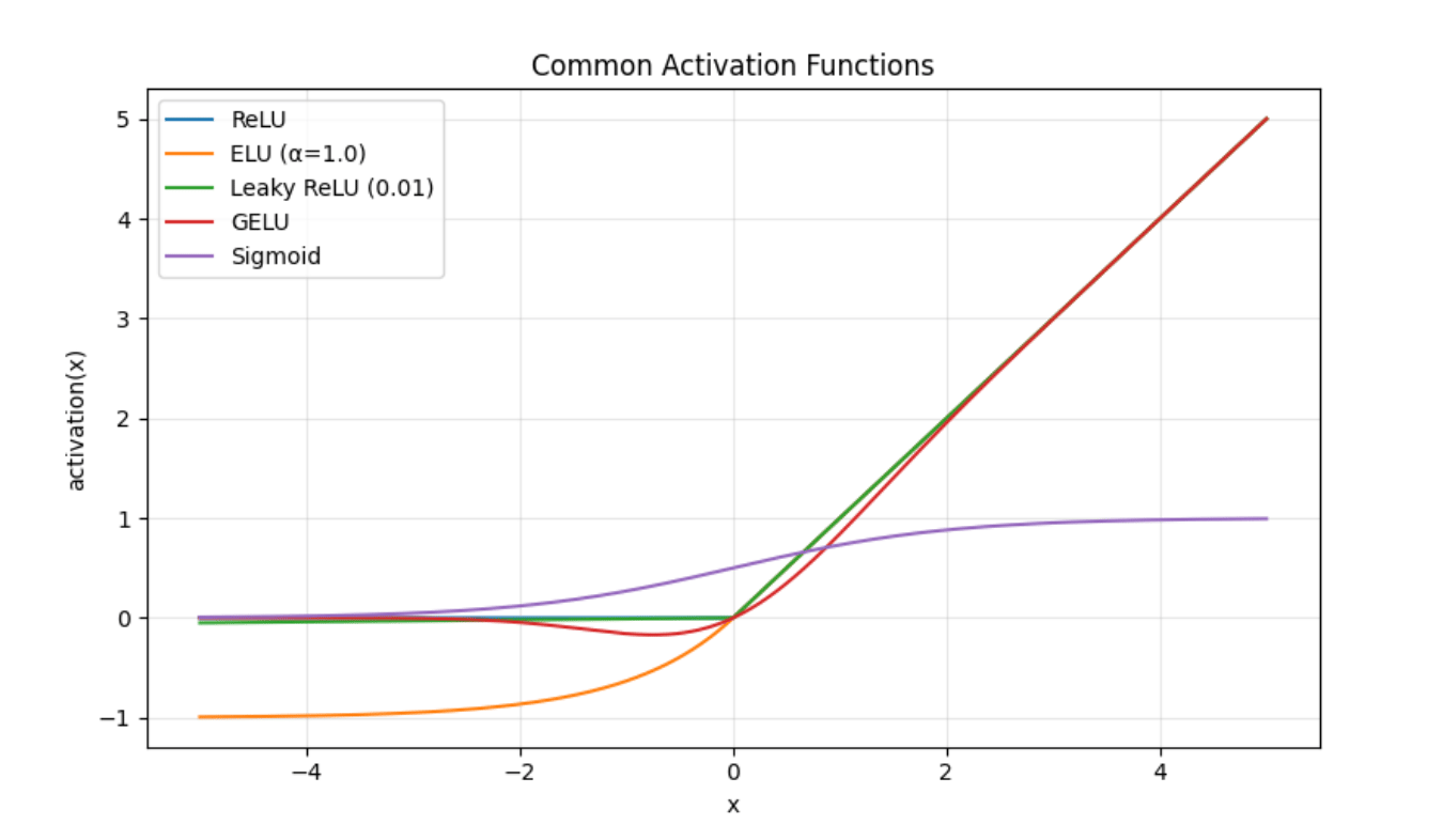
• ReLU is zero when x<0 and linear with x>0 (fast, sparse, prone to dead units).
• ELU (α=1) smoothly dips negative and saturates near −1, but has a non-zero slope when x<0 (helps center bias, has fewer dead units).
• Leaky ReLU (0.01) is almost a ReLU but has a small negative slope (avoids dead units at low cost).
• GELU is smooth, and S-shaped around 0 (probabilistically gates inputs, popular in transformers).
• Sigmoid squashes to (0,1) and saturates at the extremes (used to model probabilities, but may cause vanishing gradients in deep hidden layers).

This experiment in PyTorch compares two widely used activation functions for deep neural networks, ReLU and ELU, in several settings with and without Batch Normalization. It uses a synthetic dataset and records training metrics and activation statistics. This should provide intuition on when to use each of them.

1) Import Necessary Libraries

We will use the following libraries:

• time: for measuring runtime/performance.
• torch: The PyTorch core library.
• torch.nn: Components for building neural networks (layers, activations, etc. ).
• DataLoader and TensorDataset: For handling training/validation data batches.

import time
import torch
import torch.nn as nn
from torch.utils.data import DataLoader, TensorDataset

2. Create a Synthetic Dataset with make_data

In the code below:

• We generate synthetic input features X with a negative shift to bias the ReLU activations.
• Random weights W are generated to create logits (class scores).
• Labels y are the index of the largest logit score per sample.
• The random data is split into training and validation using PyTorch TensorDatasets.

# ----------------------------
# Data: synthetic but non-trivial
# ----------------------------
def make_data(n_train=6000, n_val=2000, d=64, k=10, seed=0, shift=-1.0):
    g = torch.Generator().manual_seed(seed)
    X = torch.randn(n_train + n_val, d, generator=g) + shift  # bias negatives to stress ReLU
    W = torch.randn(d, k, generator=g) * 0.7
    logits = X @ W + 0.3 * torch.randn(n_train + n_val, k, generator=g)
    y = torch.argmax(logits, dim=1)
    X_train, X_val = X[:n_train], X[n_train:]
    y_train, y_val = y[:n_train], y[n_train:]
    train = TensorDataset(X_train, y_train)
    val = TensorDataset(X_val, y_val)
    return train, val

3. Define Multi-Layer Perceptron (MLP) Model Class

The PyTorch MLP code below is a “controlled testbed” for activation ablations. We keep the architecture fixed and only change the nonlinearity (ReLU/ELU) and the optional BatchNorm toggle.

It is defined with two identical hidden blocks Linear → (BatchNorm) → Activation (note BatchNorm before nonlinearity), followed by a linear head layer to output raw logits. ELU’s alpha is configurable. We explicitly set ReLU/ELU to be inplace=False for safe autograd. We initialize all linear layers with He/Kaiming (fan-in, nonlinearity=“relu”), which is the proper choice for ReLU-like activations, including ELU.

# PyTorch MLP with switchable activation (ReLU | ELU) and optional BatchNorm
# The goal is to keep the architecture identical while toggling just the nonlinearity
# and BN, so training differences reflect activation choice rather than #model capacity.


# ----------------------------
# Model: same MLP, toggled activation and BatchNorm
# ----------------------------
class MLP(nn.Module):
    """
    Minimal MLP for controlled activation ablations.

    Args:
        in_dim:   Input feature dimension (expects x of shape [B, in_dim]).
        hidden:   Width of hidden layers (two identical hidden blocks are used).
        out_dim:  Output dimension (e.g., number of classes; logits are returned).
        act:      'relu' or 'elu' -- activation used in all hidden blocks.
        use_bn:   If True, apply BatchNorm1d after each Linear (before activation).
        alpha:    ELU shape parameter (ignored when act='relu').

    Notes:
        - Final layer has NO activation/BN to return raw logits. Apply softmax/sigmoid
          outside depending on your loss (e.g., CrossEntropy expects logits).
        - He/Kaiming init is used and works well for ReLU-like activations, including ELU.
        - inplace=False keeps autograd graphs clean (safer for hooks/checkpointing).
    """
    def __init__(
        self,
        in_dim: int,
        hidden: int,
        out_dim: int,
        act: Literal["relu", "elu"] = "relu",
        use_bn: bool = False,
        alpha: float = 1.0,
    ):
        super().__init__()
        self.act_kind = act
        self.alpha = alpha
        self.use_bn = use_bn

        def block(in_f: int, out_f: int):
            """
            One hidden block: Linear -> (optional BN) -> Activation

            BN (if enabled) is placed BEFORE the nonlinearity, which is the conventional
            choice for ReLU/ELU in feed-forward nets. This helps stabilize feature scales.
            """
            layers = [nn.Linear(in_f, out_f)]
            if use_bn:
                layers.append(nn.BatchNorm1d(out_f))  # zero-mean, #unit-variance per feature
            if act == "relu":
                layers.append(nn.ReLU(inplace=False))  # cheap, sparse; can #produce dead units
            elif act == "elu":
                layers.append(nn.ELU(alpha=alpha, inplace=False))  # #smoother, neg tail to -alpha
            else:
                raise ValueError("act must be 'relu' or 'elu'")
            return layers

        # Stack two identical hidden blocks to make differences in #activations visible.
        layers = []
        layers += block(in_dim, hidden)
        layers += block(hidden, hidden)

        # Final linear "head" produces logits; keep it clean (no #BN/activation here).
        layers += [nn.Linear(hidden, out_dim)]
        self.net = nn.Sequential(*layers)

        # He/Kaiming init: good default for ReLU-like activations (fan_in scaling).
        # Using nonlinearity='relu' is standard; works fine for ELU in #practice.
        for m in self.modules():
            if isinstance(m, nn.Linear):
                nn.init.kaiming_normal_(m.weight, nonlinearity="relu")
                if m.bias is not None:
                    nn.init.zeros_(m.bias)

    def forward(self, x: torch.Tensor) -> torch.Tensor:
        """
        Forward pass.

        Expects x of shape [B, in_dim]. If your data has extra spatial dims
        (e.g., images), flatten before calling or wrap this class with a feature
        extractor. Returns raw logits of shape [B, out_dim].
        """
        return self.net(x)

4. Track Activation Statistics with ActStats

The code below tracks the health of hidden-layer activations during training, without the memory cost of storing full tensors or the maintenance cost of breaking autograd. At each batch, it updates simple aggregates (mean activation, mean absolute activation) to capture centering, drift, and scale. The class automatically infers layer width on first use, cleanly resets at each epoch start, and supports activations with size [B, H] (or anything that can flatten to that). All updates are contained within @torch.no_grad() to ensure zero overhead on gradients.

The utility then tracks branch-specific signals. For ReLU, this is the fraction of exact zeros, and the number of “dead units” that never fire. For ELU/Leaky (or any negative-branch activation), it estimates the fraction of values that are near the lower limit −α, both in terms of batch fraction and per-unit frequency, to flag units “often saturated” that are near −α in ≥90% of batches. The summary() method exposes these averages as a loggable dict for dashboards or training reports.

class ActStats:
    """
    Lightweight running stats tracker for layer activations.

    Tracks per-batch aggregates so you can monitor:
      - mean_activation:      average activation value across batches
      - mean_abs_activation:  average absolute activation value
      - ReLU-specific:
          * frac_zeros:       fraction of outputs that are exactly zero
          * dead_units:       count of hidden units that were never nonzero
      - ELU/Leaky/other-with-negative-branch:
          * frac_near_neg_saturation: fraction of outputs sitting near −alpha
          * units_often_saturated:    count of units that are 'near −alpha' ≥90% of batches

    Args:
        kind:  "relu" or anything else (treated as having a negative branch with scale `alpha`)
        alpha: scale used to detect negative saturation (e.g., ELU/LeakyReLU slope/limit)
        width: optional number of hidden units (H). If None, inferred on first update().
    """

    def __init__(self, kind, alpha=1.0, width=None):
        self.kind = kind
        self.alpha = alpha
        self.width = width
        self.reset_epoch(width)

    def reset_epoch(self, width=None):
        """
        Clear running counters at the start of an epoch (or whenever you like).
        Optionally reset the known layer width.
        """
        if width is not None:
            self.width = width

        # Batch-level accumulators
        self.n_batches = 0
        self.sum_mean = 0.0          # sum of batch means (for overall mean)
        self.sum_absmean = 0.0       # sum of batch |mean|s (for overall abs mean)

        # Kind-specific accumulators
        self.sum_zero_frac = 0.0     # ReLU: fraction of exact zeros per batch
        self.sum_negsat_frac = 0.0   # non-ReLU: fraction near negative saturation per batch

        # Per-unit trackers (initialized lazily if width unknown)
        self.unit_any_active = torch.zeros(self.width or 1, dtype=torch.bool)   # ReLU: was unit ever nonzero?
        self.unit_negsat_counts = torch.zeros(self.width or 1, dtype=torch.long) # non-ReLU: #batches this unit was near −alpha
        self.unit_total_batches = 0  # denominator for saturation frequency #per unit

    @torch.no_grad()
    def update(self, act):
        """
        Ingest a batch of activations and update running statistics.

        Args:
            act: a tensor shaped [B, H] (or anything that can be flattened to that),
                 where B = batch size, H = hidden width.
        """
        # Ensure shape [B, H]
        if act.dim() != 2:
            act = act.view(act.shape[0], -1)

        B, H = act.shape

        # Lazily finalize width-dependent buffers if needed
        if self.width is None:
            self.width = H
            self.unit_any_active = torch.zeros(H, dtype=torch.bool)
            self.unit_negsat_counts = torch.zeros(H, dtype=torch.long)

        # ---- Batch aggregates ----
        self.n_batches += 1
        self.sum_mean += act.mean().item()
        self.sum_absmean += act.abs().mean().item()

        # ---- Kind-specific tracking ----
        if self.kind == "relu":
            # ReLU: zeros signal inactivity; good to monitor dead units
            zero_frac = (act == 0).float().mean().item()
            self.sum_zero_frac += zero_frac

            # Mark units that were nonzero at least once in this batch
            # .any(dim=0) -> shape [H], True if that unit fired for any sample
            self.unit_any_active |= (act != 0).any(dim=0).cpu()

        else:
            # For ELU-/Leaky-like activations, watch negative saturation:
            # we call it "near saturation" if value < -0.95 * alpha
            # (heuristic: close to the lower branch limit)
            threshold = -0.95 * self.alpha
            near_sat_mask = (act < threshold)
            negsat_frac = near_sat_mask.float().mean().item()
            self.sum_negsat_frac += negsat_frac

            # Per-unit: how often this unit spends >50% of the batch near saturation
            near_sat_per_unit = near_sat_mask.float().mean(dim=0)  # [H], fraction in this batch
            self.unit_negsat_counts += (near_sat_per_unit > 0.5).to(torch.long).cpu()
            self.unit_total_batches += 1

    def summary(self):
        """
        Return a dict with averaged metrics over all seen batches.
        """
        out = {
            "mean_activation": self.sum_mean / max(1, self.n_batches),
            "mean_abs_activation": self.sum_absmean / max(1, self.n_batches),
        }

        if self.kind == "relu":
            out["frac_zeros"] = self.sum_zero_frac / max(1, self.n_batches)
            # Dead = never fired (still False in unit_any_active)
            out["dead_units"] = int((~self.unit_any_active).sum().item())
        else:
            out["frac_near_neg_saturation"] = self.sum_negsat_frac / max(1, self.n_batches)

            if self.unit_total_batches > 0:
                # "often saturated" = in >90% of batches, this unit was >50% near −alpha
                freq = self.unit_negsat_counts / self.unit_total_batches  # per-unit frequency
                out["units_often_saturated"] = int((freq > 0.9).sum().item())
            else:
                out["units_often_saturated"] = 0

        return out

5. Helper: Find First Activation Module in the Model

This module finds the first instance of nn.ReLU or nn.ELU in a model (if present), or returns None.

def get_first_activation_module(model):
    for m in model.modules():
        if isinstance(m, (nn.ReLU, nn.ELU)):
            return m
    return None

6. Train and Evaluate MLP Model

The code below:

• Seeds the environment, creates the dataset, and PyTorch DataLoaders.

• Creates the MLP using the selected activation and batch norm.

• Set up SGD optimizer and cross-entropy loss.

• Registers a forward hook on the first activation layer to record activation data.

• Trains the model for the specified number of epochs:

  • Performs gradient computation and weight updates.
  • Logs training loss and gradient norms.

• Evaluates validation accuracy after each epoch.

• Summarizes activations to detect dead neurons or saturation behaviors.

• Measures inference latency on a random input for timing analysis.

• Cleans up by removing the hook to prevent side effects.

# ----------------------------
# Train & evaluate one setting
# ----------------------------
def run_experiment(act="relu", use_bn=False, alpha=1.0, seed=0,
                   in_dim=64, hidden=256, out_dim=10, epochs=10, batch_size=128, lr=1e-1):
    torch.manual_seed(seed)
    train_ds, val_ds = make_data(d=in_dim, k=out_dim, seed=seed, shift=-1.0)
    train_dl = DataLoader(train_ds, batch_size=batch_size, shuffle=True)
    val_dl = DataLoader(val_ds, batch_size=512, shuffle=False)

    model = MLP(in_dim, hidden, out_dim, act=act, use_bn=use_bn, alpha=alpha)
    device = torch.device("cuda" if torch.cuda.is_available() else "cpu")
    model.to(device)

    opt = torch.optim.SGD(model.parameters(), lr=lr, momentum=0.9)
    loss_fn = nn.CrossEntropyLoss()

    # Hook to capture activation stats on the first hidden activation
    act_mod = get_first_activation_module(model)
    width = hidden
    tracker = ActStats(kind=act, alpha=alpha, width=width)

    def hook_fn(module, inp, out):
        tracker.update(out.detach())

    hook_handle = act_mod.register_forward_hook(hook_fn) if act_mod else None

    epoch_times, train_losses, val_accs, grad_norms = [], [], [], []

    for ep in range(1, epochs + 1):
        tracker.reset_epoch(width)
        t0 = time.perf_counter()
        model.train()
        running = 0.0
        batches = 0
        grad_norm_sum = 0.0
        for xb, yb in train_dl:
            xb, yb = xb.to(device), yb.to(device)
            opt.zero_grad(set_to_none=True)
            logits = model(xb)
            loss = loss_fn(logits, yb)
            loss.backward()
            first_layer = model.net[0]
            gn = first_layer.weight.grad.norm().item()
            grad_norm_sum += gn
            opt.step()
            running += loss.item()
            batches += 1

        epoch_time = time.perf_counter() - t0
        epoch_times.append(epoch_time)
        train_losses.append(running / max(1, batches))
        grad_norms.append(grad_norm_sum / max(1, batches))

        # Validation
        model.eval()
        correct, total = 0, 0
        with torch.no_grad():
            for xb, yb in val_dl:
                xb, yb = xb.to(device), yb.to(device)
                pred = model(xb).argmax(dim=1)
                correct += (pred == yb).sum().item()
                total += yb.numel()
        val_acc = correct / max(1, total)
        val_accs.append(val_acc)

        # Activation summary for this epoch
        act_summary = tracker.summary()

        print(f"[act={act.upper()} | BN={'ON' if use_bn else 'OFF'}] "
              f"Epoch {ep:02d} | loss {train_losses[-1]:.4f} | val_acc {val_acc:.3f} | "
              f"grad|| {grad_norms[-1]:.3f} | time {epoch_time*1000:.0f} ms")
        if act == "relu":
            print(f"    mean_act {act_summary['mean_activation']:.3f} | "
                  f"%zeros {100*act_summary['frac_zeros']:.1f}% | "
                  f"dead_units {act_summary['dead_units']}")
        else:
            print(f"    mean_act {act_summary['mean_activation']:.3f} | "
                  f"%near(-alpha) {100*act_summary['frac_near_neg_saturation']:.1f}% | "
                  f"units_often_saturated {act_summary['units_often_saturated']}")

    # Inference latency (forward pass only)
    with torch.no_grad():
        xb = torch.randn(1024, in_dim, device=device)
        t1 = time.perf_counter()
        _ = model(xb)
        fwd_ms = (time.perf_counter() - t1) * 1000

    if hook_handle:
        hook_handle.remove()

    return {
        "train_loss": train_losses,
        "val_acc": val_accs,
        "epoch_time_ms": sum(epoch_times) / len(epoch_times),
        "grad_norm_first": sum(grad_norms) / len(grad_norms),
        "fwd_ms_1024": fwd_ms,
    }

7. Helper to Format Summary Rows for Printing

This will include final validation accuracy alongside average epoch time, forward latency, and average gradient norm.

def pretty_row(name, stats):
    return (f"{name:22s} | "
            f"final_acc {stats['val_acc'][-1]:.3f} | "
            f"avg_epoch {stats['epoch_time_ms']:.0f} ms | "
            f"fwd(1024) {stats['fwd_ms_1024']:.1f} ms | "
            f"grad|| {stats['grad_norm_first']:.3f}")

8. Main Experiment Entry Point

The script below:

• Runs two experiments for both activations:

• Without BatchNorm (Regime A) which ELU can help avoid dead neurons.

• With BatchNorm (Regime B) where ReLU is typically faster and performs well.

• Prints out informative summary comparisons.

if __name__ == "__main__":
    EPOCHS = 10
    HIDDEN = 256
    SEED = 0
    LR = 1e-1
    ALPHA = 1.0

    print("\n=== Regime A: NO BatchNorm (where ELU often helps) ===")
    stats_relu_noBN = run_experiment(act="relu", use_bn=False, alpha=ALPHA, seed=SEED,
                                     hidden=HIDDEN, epochs=EPOCHS, lr=LR)
    stats_elu_noBN  = run_experiment(act="elu",  use_bn=False, alpha=ALPHA, seed=SEED,
                                     hidden=HIDDEN, epochs=EPOCHS, lr=LR)

    print("\nSummary (No BatchNorm):")
    print(pretty_row("ReLU (no BN)", stats_relu_noBN))
    print(pretty_row("ELU  (no BN)", stats_elu_noBN))

    print("\n=== Regime B: WITH BatchNorm (where ReLU often wins on speed) ===")
    stats_relu_BN = run_experiment(act="relu", use_bn=True, alpha=ALPHA, seed=SEED,
                                   hidden=HIDDEN, epochs=EPOCHS, lr=LR)
    stats_elu_BN  = run_experiment(act="elu",  use_bn=True, alpha=ALPHA, seed=SEED,
                                   hidden=HIDDEN, epochs=EPOCHS, lr=LR)

    print("\nSummary (With BatchNorm):")
    print(pretty_row("ReLU (BN on)", stats_relu_BN))
    print(pretty_row("ELU  (BN on)", stats_elu_BN))

    print("\nInterpretation:")
    print("- No BN: if ReLU shows many dead units / high %zeros and ELU trains steadier with zero-mean-ish activations, prefer ELU.")
    print("- With BN: if accuracy is similar but ReLU is faster per epoch and at inference, prefer ReLU.")

Example of summary row

Summary (No BatchNorm):
ReLU (no BN) | final_acc 0.860 | avg_epoch 0 ms | fwd(1024) 7.5 ms | grad|| 1.067
ELU  (no BN) | final_acc 0.500 | avg_epoch 1 ms | fwd(1024) 11.8 ms | grad|| 1.867

Interpretation:

• final_acc: validation accuracy after the last epoch.
• avg_epoch: average time per epoch (training speed).
• fwd(1024): Inference latency with a batch of 1024 samples.
• grad||: average L2 norm of first layer weight gradients (approximate learning signal).

How to interpret typical outcomes

• No BatchNorm:
  • If ReLU has a high percentage of zeros output / dead units, and accuracy is poor or loss is noisy, then try ELU.
  • If ELU is showing moderate near-saturation, but trains stably with acceptable accuracy, it did its job.
• With BatchNorm:
  • Accuracy between ReLU and ELU typically ends up similar.
  • ReLU is faster during training and inference—use it if latency/throughput are critical.
  • If ELU isn’t clearly helping accuracy, use ReLU + BN for simplicity/speed.

• Initialization: It is common practice to use He/Kaiming initialization for ReLU, because it properly accounts for the behavior of ReLU in the forward/backward passes. For ELU, you can also apply Kaiming initialization with nonlinearity=‘relu’. However, you can also tune the gain slightly lower, since ELU’s variance properties are somewhat different from ReLU’s.
• Alpha for ELU: The standard is α=1.0. Higher α increases the magnitude of the negative saturation region, which further pulls means closer to zero but may slightly affect the scale of gradients.
• BatchNorm interaction: When using BatchNorm after each block, ELU’s zero-mean property is not required, as the BatchNorm will normalize the activation distribution. In those networks, benchmark with ReLU first, and only consider switching to ELU if you experience instabilities.
• In-place ops: In PyTorch, inplace=True can save memory but causes issues with autograd on exotic computation graphs. If you see strange errors, try setting inplace=False.
• Quantization: ReLU tends to be more friendly to integer quantization pipelines (widely used in mobile/embedded). ELU can also be used, but may have different accuracy/speed tradeoffs, so be sure to test with your quantizer.

• Convergence speed: ELU’s zero-centering can provide a modest speed-up to early training or result in more stable training on some tasks, particularly in the absence of BatchNorm. On the other hand, BatchNorm typically shrinks these differences in practice.
• Final accuracy: ReLU and ELU have mostly been found to have roughly the same ceiling on performance on many vision and tabular tasks. When differences exist, ELU can have the edge in noisier/unnormalized settings, while ReLU can win when its simplicity/speed allows for iteration and testing with more architectures/regularization ideas.
• Dead units: A risk of ReLU is that if the units’ weights drift too far negative, they start outputting zero all the time, and never recover. The negative slope of ELU units allows gradients to keep flowing, reducing the risk of dead units. Leaky ReLU presents a cost-effective alternative for avoiding exponential calculations by allowing limited gradients to pass through negative values.
• Robustness to outliers: ELU alleviates the impact of extreme negative values by asymptotically saturating to a fixed negative value. This makes ELU more robust in the presence of outliers and heavy-tailed data than ReLU, which aggressively zeroes out all negative values.
• Hardware/latency: ReLU has a lower computational cost and latency during inference, since it’s simply a max operation. ELU is slightly more expensive with its exponential function. That makes it faster and more stable during training in some contexts.

• Use ELU when
  • Training is unstable or slow to converge with ReLU (especially without BatchNorm).
  • You see many “dead” ReLU units or poor negative-region gradients.
  • You want zero-centered activations while being able to manage a slight increase in computational expense.
  • Negative activations can be useful for regression tasks that involve symmetric targets.
• Use ReLU when…
  • You require the fastest operational speed and simple deployment (edge/mobile).
  • You already rely heavily on BatchNorm; the zero-centering gain of ELU may not have a big impact.
  • Your model is shallow-to-moderate.
  • Tooling or quantization constraints favor piecewise linear operations.
• Consider Leaky ReLU if…
  • You want a cost-effective solution to prevent dying ReLU units without using exponential functions.
  • You like ReLU’s fast computation speed but desire a mechanism to handle negative activations.
• Consider GELU if…
  • You’re in Transformer-like architecture where GELU has become the standard.

• Q1. Does ELU always outperform ReLU? No. In many applications, ELU has faster early convergence or better stability. However, when both models are well tuned (BatchNorm, LR schedules), their final accuracy can be similar. Always benchmark for your dataset.

• Q2. What α should I use for ELU? α=1 is standard and works well in most cases. Manually tuning α gives diminishing returns, unless you have a good distributional reason for doing so.

• Q3. Is Leaky ReLU a better compromise? Often. Leaky ReLU removes dead neurons without significant performance trade-offs when compared to ReLU. If the additional smoothness of ELU fails to deliver improved stability or other benefits, Leaky ReLU is a strong default.

• Q4. Why is GELU popular if it’s slower? It works very well empirically in transformer architectures. If your model family typically uses GELU (BERT/ViT variants), then use it as a black-box component and accept the additional computation as a reasonable trade-off for the performance gain.

• Q5. ReLU vs sigmoid—why not sigmoid? The sigmoid saturates at both ends (near 0 and 1). When it is in the saturated region, the derivative is close to zero, and therefore gives rise to a very small gradient. This will result in slow or no weight update during backpropagation. This is more problematic when there are deep stacks of hidden layers. Thus, the sigmoid activation function is not recommended within hidden neural network layers to prevent the vanishing gradient problem.

Conclusion

ReLU remains a fast, reliable baseline. ELU sacrifices some compute for smoother optimization, fewer dead units, and often faster early convergence. In practice, you’ll get the most salient signal by benchmarking both under the same seed, schedule, and hardware, and—if latency is a concern—adding Leaky ReLU to the mix. For transformer-style stacks, GELU will usually be the right choice. Whichever you choose, be sure to measure on your data and maintain the same initialization, normalization, and learning-rate policy across trials.

The Gradient AI platform from DigitalOcean provides a convenient solution for experiments through GPU notebooks, job runners, and deployable endpoints. This will make it easy to spin up notebooks, track results, and push trained models into production without rebuilding your stack.

• Vanishing and Exploding Gradients Problems in Deep Learning
• FAST AND ACCURATE DEEP NETWORK LEARNING BY EXPONENTIAL LINEAR UNITS (ELUS)
• Activation Functions
• Variants of ReLU (Leaky ReLU, PReLU, ELU)
• Tutorial 2: Activation Functions