By Adrien Payong and Shaoni Mukherjee

Manually optimizing machine learning parameters involves adjusting model settings through trial-and-error to enhance performance. Through manual machine learning parameter tuning, you can develop a better understanding of your model’s functionality. This guide will show you how to manually optimize machine learning models.
We will provide multiple model tuning methods, including one-at-a-time tuning, manual grid search, and random search techniques. We will also provide Python code examples that demonstrate learning rate tuning techniques and performance evaluation methods.
Prerequisites
- Confidently write and run Python scripts while managing library installations.
- Practical experience with scikit-learn for training and evaluating machine learning models such as SVC and GradientBoostingClassifier.
- Understanding the distinction between model parameters and hyperparameters, training/validation/test sets, and evaluation metrics like accuracy, F1-score, and AUC.
- A Python environment where numpy, pandas, matplotlib, and scikit-learn libraries are installed.
- Comfort with concepts like bias-variance trade-off, loss functions, and gradient-based optimization.
Model Parameters vs. Hyperparameters
Model parameters represent the internal weights or coefficients that a machine learning model learns from data during training. These directly influence predictions (e.g., the prediction of a neural network depends on its learned weights).
On the other hand, model hyperparameters represent external configurations that users manually set to direct the machine learning training. They remain constant throughout training because they guide the learning process instead of being learned from the data.
Why Tune Hyperparameters Manually?
Current machine learning libraries provide automated hyperparameter tuning capabilities. However, manual hyperparameter tuning can be useful in some specific situations. Let’s consider some of them:
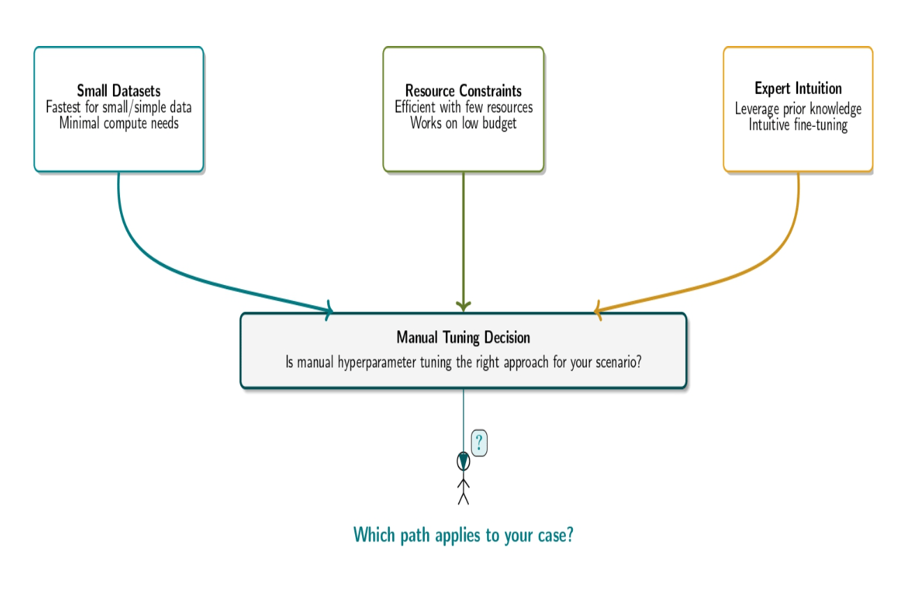
Small Datasets or Simple Models
When dealing with small problems or basic algorithms, manual hyperparameter tuning can be the fastest approach. Automated methods may be overkill. Manually tuning parameters can be useful for small datasets or basic models, despite being time-intensive.
Resource Constraints
Automated hyperparameter search requires extensive computational power because it tries many possible combinations. Selective manual exploration of a few settings enables the development of an adequate model when resources are limited.
Expert Intuition
Practitioners with experience often have intuition about which hyperparameter ranges work well based on theoretical insights or previous experience. Using intuition to search hyperparameter values manually can achieve better solutions more quickly compared to automated blind searches.
Manual Hyperparameter Tuning for SVM: A Step-by-Step Guide
Let’s consider a binary classification problem (e.g., classifying tumors as benign vs malignant). We will use the scikit-learn Breast Cancer Wisconsin dataset for our analysis. We will also implement a support vector machine classifier using its default configuration settings.
Establish a Baseline Model
Start by training a baseline model using the default hyperparameters. A baseline model allows you to establish a reference point by showing basic performance statistics upon which to improve. Let’s consider the following code:
from sklearn.datasets import load_breast_cancer
from sklearn.model_selection import train_test_split
from sklearn.svm import SVC
from sklearn.metrics import accuracy_score, f1_score, roc_auc_score

# Load dataset and split into train/validation sets
X, y = load_breast_cancer(return_X_y=True)
X_train, X_val, y_train, y_val = train_test_split(
    X, y, test_size=0.2, random_state=42, stratify=y
)

# Train a baseline SVM model with default hyperparameters
model = SVC(kernel='rbf', probability=True, random_state=42)
model.fit(X_train, y_train)
y_pred = model.predict(X_val)

# Evaluate baseline performance
print("Baseline accuracy:", accuracy_score(y_val, y_pred))
print("Baseline F1-score:", f1_score(y_val, y_pred))
print("Baseline AUC:", roc_auc_score(y_val, model.predict_proba(X_val)[:, 1]))
Output:
Baseline accuracy: 0.9298245614035088
Baseline F1-score: 0.9459459459459459
Baseline AUC: 0.9695767195767195
The model demonstrates a 92% validation classification accuracy using default parameters, while the F1-score (~0.94) reflects a good precision-recall balance. AUC (~0.96) shows excellent ranking performances. You can use these metrics as the baseline for comparison.
Why multiple metrics? Accuracy alone can be misleading, especially with imbalanced data. Our evaluation incorporates F1-score to balance precision/recall, along with AUC to rank performance over all classification thresholds. You can choose the metric that is aligned with your objective (such as F1 or AUC).
Choose Hyperparameters to Tune
Although models typically feature multiple settings, they are not equally important. The best practice is to focus initially on a limited number of key hyperparameters. For our SVM example, we will focus on two major hyperparameters, which are C and gamma.
-
C (Regularization parameter): Controls the trade-off between model complexity and error on training data.
- Low C: The model applies stronger regularization, which can cause higher bias but reduce variance, increasing the risk of underfitting.
- High C: Weaker regularization, allowing the model to fit the training data more closely. This reduces bias but increases variance, increasing the risk of overfitting.
-
Gamma (Kernel coefficient): This determines how much influence a single training example has on the decision boundary.
- Low gamma: Points have broader influence, resulting in smoother, more generalized decision boundaries.
- High gamma: Each point impacts only its immediate neighborhood, which can lead to complex boundaries.
Tune Hyperparameters One-by-One (Manual Trial and Error)
You can adjust one key hyperparameter at a time to see how the model responds. Hyperparameter tuning can start with manual trial-and-error, which is the simplest tuning method.
Procedure:
- Start your experiments by choosing a single hyperparameter to adjust (such as C in SVM models).
- Choose a series of candidate values for testing based either on intuition or default settings. Hyperparameters often show non-linear effects, which makes it beneficial to test C values on a logarithmic scale(e.g., 0.01, 0.1, 1, 10, 100).
- For each selected value, train the model and evaluate its performance on the validation set.
- Plot or print the results to determine the best value before choosing it as your starting point.
Let’s consider the following example:
for C in [0.01, 0.1, 1, 10, 100]:
    model = SVC(kernel='rbf', C=C, probability=True, random_state=42)
    model.fit(X_train, y_train)
    val_ac = accuracy_score(y_val, model.predict(X_val))
    print(f"C = {C:<5} | Validation Accuracy = {val_ac:.3f}")
Output:
C = 0.01  | Validation Accuracy = 0.842
C = 0.1   | Validation Accuracy = 0.912
C = 1     | Validation Accuracy = 0.930
C = 10    | Validation Accuracy = 0.930
C = 100   | Validation Accuracy = 0.947
Low C (e.g., 0.01) results in under-regularization → underfitting (low accuracy).
Moderate C (around 1) often achieves an effective balance between bias and variance.
Very high C (e.g., 100) may lead to minor overfitting, which sometimes increases accuracy but reduces generalization ability.
Next, you could fix C=1 and tune gamma similarly:
for gamma in [1e-4, 1e-3, 1e-2, 0.1, 1]:
    model = SVC(kernel='rbf', C=1, gamma=gamma, probability=True, random_state=42)
    model.fit(X_train, y_train)
    val_ac = accuracy_score(y_val, model.predict(X_val))
    print(f"gamma = {gamma:<6} | Validation Accuracy = {val_ac:.3f}")
Output:
gamma = 0.0001 | Validation Accuracy = 0.930
gamma = 0.001  | Validation Accuracy = 0.895
gamma = 0.01   | Validation Accuracy = 0.640
gamma = 0.1    | Validation Accuracy = 0.632
gamma = 1      | Validation Accuracy = 0.632
γ = 1e-4: Low γ values produce straightforward decision boundaries that prevent overfitting while delivering the highest accuracy of 0.930. γ ≥ 1e-3: As γ increases, the RBF kernel becomes more sensitive to individual points and risks overfitting, which reduces generalization capability as shown by the significant accuracy drop to ~0.895 and below.
Key Takeaways
- Manual one-at-a-time tuning helps you to build intuition about hyperparameters’ effects.
- Use the validation set for hyperparameter selection and keep the test set for final evaluation to avoid overfitting.
- Using multiple evaluation metrics(Such as F1 and AUC) for robust evaluation can help to identify overfitting and bias/variance issues at early stages.
After identifying promising hyperparameter ranges through manual tuning, you can proceed with systematic search approaches like manual grid search, random search, or Bayesian optimization.
Manual Grid Search (Systematic Exploration)
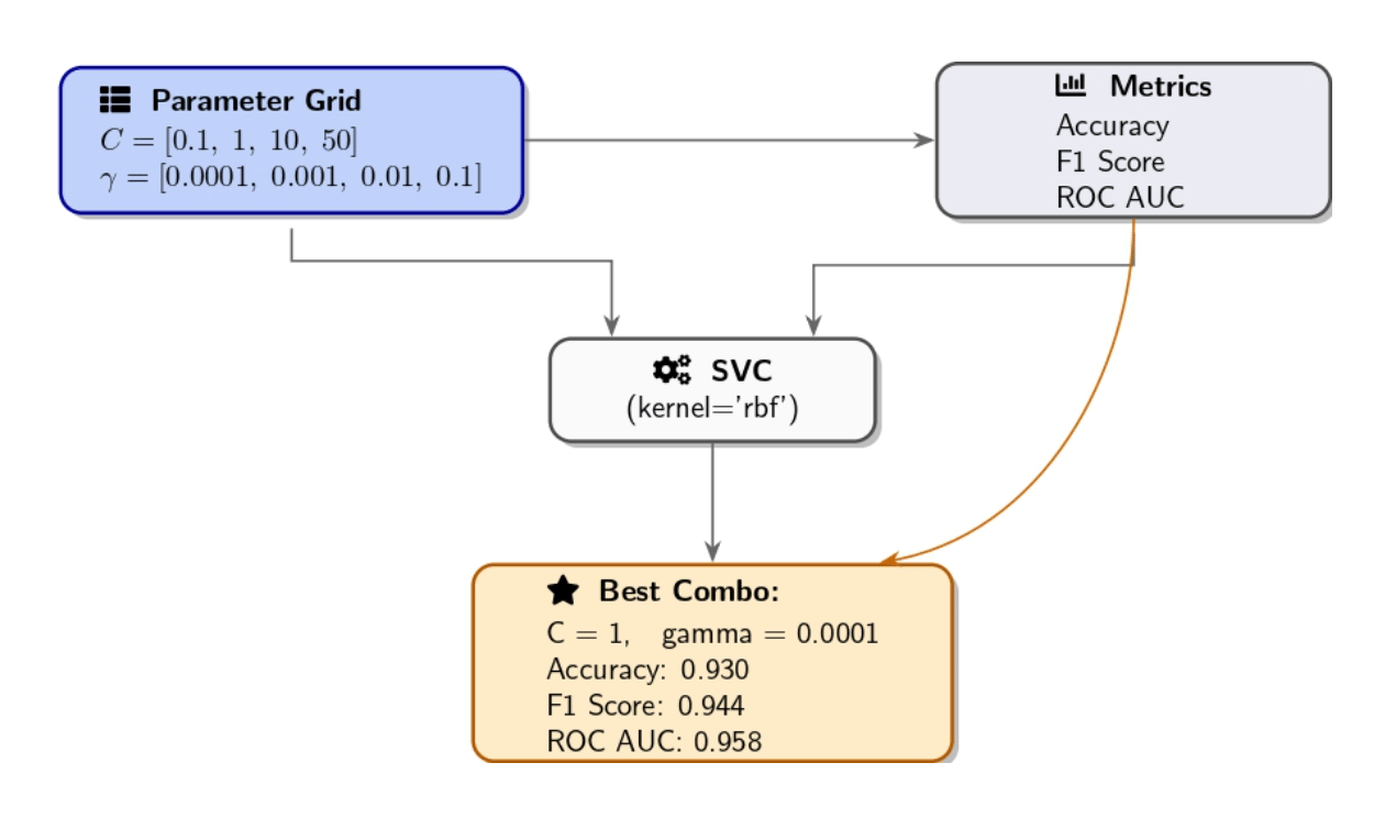
After performing initial one-by-one explorations, a manual grid search will allow you to explore combinations of hyperparameters. The grid search approach involves setting up a grid of potential values for each hyperparameter before evaluating each combination against the model. Our approach included sweeping C over 0.1, 1, 10, 50, and γ ranged between 1e−4, 1e−3, 0.01, 0.1 as we trained an RBF-kernel SVM for each pair combination. We then evaluate their performance using the validation set. The combination of (C, γ) parameters that produces the highest validation accuracy was selected as our best_params while also tracking F1/AUC.
from sklearn.metrics import accuracy_score, f1_score, roc_auc_score

param_grid = {
    "C":     [0.1, 1, 10, 50],
    "gamma": [1e-4, 1e-3, 0.01, 0.1]
}

best_ac = 0.0
best_f1  = 0.0
best_auc = 0.0
best_params = {}

for C in param_grid["C"]:
    for gamma in param_grid["gamma"]:
        model = SVC(kernel='rbf',
                    C=C,
                    gamma=gamma,
                    probability=True,
                    random_state=42)
        model.fit(X_train, y_train)

        # Predictions and probabilities
        y_v_pred  = model.predict(X_val)
        y_v_proba = model.predict_proba(X_val)[:, 1]

        # metrics computation
        ac = accuracy_score(y_val, y_v_pred)
        f1  = f1_score(y_val, y_v_pred)
        auc = roc_auc_score(y_val, y_v_proba)

        # You can Track best by accuracy or change to f1/auc as needed
        if ac > best_ac:
            best_ac    = ac
            best_f1     = f1
            best_auc    = auc
            best_params = {"C": C, "gamma": gamma}

        print(f"C={C:<4}  gamma={gamma:<6}  => "
              f"Accuracy={ac:.3f}  F1={f1:.3f}  AUC={auc:.3f}")

print(
    "\nBest combo:", best_params,
    f"with Accuracy={best_ac:.3f}, F1={best_f1:.3f}, AUC={best_auc:.3f}"
)
Output:
Best combo: {'C': 1, 'gamma': 0.0001} with Accuracy=0.930, F1=0.944, AUC=0.958
The grid search matched baseline accuracy, yet the results showed slight reductions in F1 and AUC scores. This indicates that the SVM default hyperparameters are near optimal for F1/AUC, and the manual grid search was too coarse or targeted the wrong regions.
Key points for manual grid search:
- The granularity of the grid matters. A coarse grid (few values) may overlook the best possible solution. A fine grid with numerous values increases the possibility of finding the best combination, but requires more training runs.
- When dealing with a large grid, it’s beneficial to apply cross-validation for a robust evaluation of each combination, but be aware that it increases computational requirements.
- Grid search suffers from the curse of dimensionality: Increasing hyperparameters or values can explode the number of combinations. At this point, random search emerges as a valuable strategy.
Manual Random Search for Hyperparameter Optimization
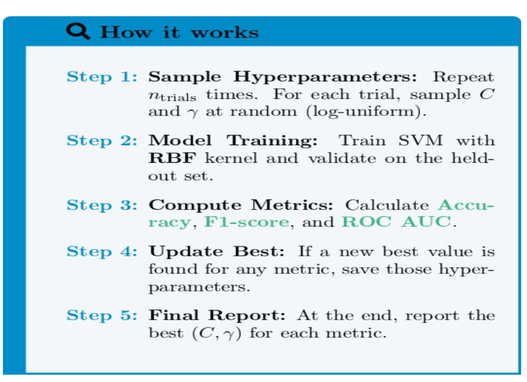
Start manual random search by selecting reasonable ranges for each hyperparameter. You can then randomly choose values within those ranges for several trials. In our experiment, we select C values from a log-uniform distribution between 0.1 and 100, and gamma values are selected between 1e-5 and 1e-2.
The function below will enable you to conduct a random search across multiple metrics. It will allow you to identify optimal hyperparameters for Accuracy, F1-Score, and ROC AUC in one pass.
import random
import numpy as np
from sklearn.svm import SVC
from sklearn.metrics import accuracy_score, f1_score, roc_auc_score

def random_search_svm(X_train, y_train, X_val, y_val, ntrials=10):
    """
    Run random search across C and gamma parameters for an RBF SVM model.
    Monitor optimal hyperparameters for peak Accuracy, F1-score, and ROC AUC values.
    """
    best = {
        'accuracy': {'score': 0, 'params': {}},
        'f1':       {'score': 0, 'params': {}},
        'auc':      {'score': 0, 'params': {}}
    }

    for i in range(1, ntrials + 1):
        # Log-uniform sampling
        C = 10 ** random.uniform(-1, 2)       # 0.1 to 100
        gamma = 10 ** random.uniform(-5, -2)  # 1e-5 to 1e-2

        # model training
        model = SVC(kernel='rbf', C=C, gamma=gamma,
                    probability=True, random_state=42)
        model.fit(X_train, y_train)

        # Prediction and evaluation
        y_pred = model.predict(X_val)
        y_proba = model.predict_proba(X_val)[:, 1]
        ac = accuracy_score(y_val, y_pred)
        f1 = f1_score(y_val, y_pred)
        auc = roc_auc_score(y_val, y_proba)

        # Print trial results
        print(f"Trial {i}: C={C:.4f}, gamma={gamma:.5f} | "
              f"Acc={ac:.3f}, F1={f1:.3f}, AUC={auc:.3f}")

        # For each metric, we will update the best
        if ac > best['accuracy']['score']:
            best['accuracy'].update({'score': ac, 'params': {'C': C, 'gamma': gamma}})
        if f1 > best['f1']['score']:
            best['f1'].update({'score': f1, 'params': {'C': C, 'gamma': gamma}})
        if auc > best['auc']['score']:
            best['auc'].update({'score': auc, 'params': {'C': C, 'gamma': gamma}})

    # For each metric, print summary of best hyperparameters
    print("\nBest hyperparameters by metric:")
    for metric, info in best.items():
        params = info['params']
        score = info['score']
        print(f"- {metric.capitalize()}: Score={score:.3f}, Params= C={params.get('C'):.4f}, gamma={params.get('gamma'):.5f}")
When calling the function random_search_svm(X_train, y_train, X_val, y_val, ntrials=20) to perform a more thorough search, you will get something like this:
Best hyperparameters by metric:
- Accuracy: Score=0.939, Params= C=67.2419, gamma=0.00007
- F1: Score=0.951, Params= C=59.5889, gamma=0.00002
- Auc: Score=0.987, Params= C=59.5889, gamma=0.00002
Note that different runs may yield different results because of randomness in trials. The results show which (C, γ) pairs achieve optimal performance across each key metric. This straightforward random search method reliably finds hyperparameter configurations that outperform existing baselines and coarse grid search results.
Evaluate Model Performance and Select the Best Model
Our validation set results show that the default RBF-SVM achieved strong baseline performance with 0.9298 accuracy, 0.9459 F1 score, and 0.9696 AUC.
Testing all combinations of C values {0.1, 1, 10, 50} with γ values {1e-4, 1e-3, 0.01, 0.1} improved the accuracy by a small margin to reach 0.9300. The coarse grid search resulted in a lower AUC of 0.9580 and F1 score of 0.9440, indicating that it may have overlooked the most suitable kernel.
In contrast, a targeted random sampling approach within ranges C ∈ [0.1, 100] and γ ∈ [1e-5, 1e-2] reveals three distinct optimal parameter settings:
- Accuracy‐optimized: C ≈ 67.24, γ ≈ 7 × 10⁻⁵ (Accuracy = 0.9390)
- F1‐optimized: C ≈ 59.59, γ ≈ 2 × 10⁻⁵ (F1 = 0.9510)
- AUC‐optimized: C ≈ 59.59, γ ≈ 2 × 10⁻⁵ (AUC = 0.9870)
This random‐search approach improved accuracy by nearly 0.01 and F1 by 0.005 over baseline, while boosting AUC by almost 0.02—a substantial enhancement in ranking performance.
Primary Objective:
- If the ultimate goal is overall correctness, choose the Accuracy-optimized model.
- Go for the F1-optimized model if balanced precision and recall matter.
- The AUC-optimized model should be selected if ranking performance across thresholds is your priority.
If you intend to deploy this model, you should retrain it on the combined training and validation data and evaluate its performance using the test set.
The code example demonstrates how to load and split the dataset and then merge training and validation partitions, refitting the model with optimal settings, and evaluating its performance on the test data using accuracy, F1-score, and ROC AUC metrics.
from sklearn.datasets import load_breast_cancer
from sklearn.model_selection import train_test_split
from sklearn.svm import SVC
from sklearn.metrics import accuracy_score, f1_score, roc_auc_score
import numpy as np

# 1. data loading and spliting into train+val vs. test
X, y = load_breast_cancer(return_X_y=True)
X_tem, X_test, y_tem, y_test = train_test_split(
    X, y, test_size=0.2, random_state=42, stratify=y
)

# 2.Spliting X_tem into training and validation sets. We want to reproduce the previous split
X_train, X_val, y_train, y_val = train_test_split(
    X_tem, y_tem, test_size=0.25, random_state=42, stratify=y_tem
)
# Note that 0.25 of 80% give us 20% validation, that matches our original 80/20 split

# 3. We merge train and validation data for our final testing
X_merged = np.vstack([X_train, X_val])
y_merged = np.hstack([y_train, y_val])

# 4. Retrain using our best hyperparameters
best_C = 59.5889      # replace with your chosen C
best_gamma = 2e-05    # replace with your chosen gamma

f_model = SVC(
    kernel='rbf',
    C=best_C,
    gamma=best_gamma,
    probability=True,
    random_state=42
)
f_model.fit(X_merged, y_merged)

# 5. Evaluate on hold-out test set
y_test_pred = f_model.predict(X_test)
y_test_proba = f_model.predict_proba(X_test)[:, 1]

test_ac = accuracy_score(y_test, y_test_pred)
test_f1 = f1_score(y_test, y_test_pred)
test_auc = roc_auc_score(y_test, y_test_proba)

print("Final model test accuracy:   ", test_ac)
print("Final model test F1-score:    ", test_f1)
print("Final model test ROC AUC:     ", test_auc)
Running this block will produce performance metrics from the hold-out test set, which show how the tuned SVM model performs on new data. You can check the final accuracy, F1, and AUC scores against the baseline and grid/random search results to confirm meaningful real-world improvements from the selected configuration.
Tuning the Learning Rate
The learning rate is a critical hyperparameter during neural network training. For illustration, let’s explore a Gradient Boosting Classifier as our model.
from sklearn.ensemble import GradientBoostingClassifier

for lr in [0.001, 0.01, 0.1, 0.3, 0.7, 1.0]:
    model = GradientBoostingClassifier(n_estimators=50, learning_rate=lr, random_state=42)
    model.fit(X_train, y_train)
    val_acc = accuracy_score(y_val, model.predict(X_val))
    print(f"Learning rate {lr:.3f} => Validation Accuracy = {val_acc:.3f}")
Output:
Learning rate 0.001 => Validation Accuracy = 0.632
Learning rate 0.010 => Validation Accuracy = 0.939
Learning rate 0.100 => Validation Accuracy = 0.947
Learning rate 0.300 => Validation Accuracy = 0.956
Learning rate 0.700 => Validation Accuracy = 0.956
Learning rate 1.000 => Validation Accuracy = 0.965
At a learning rate of 0.001, the model advances too slowly to improve performance. The model’s accuracy shows improvement once we adjust the learning rate to 0.1 or higher. When the learning rate is set between 0.3 to 1.0, we achieve high performance levels, reaching about 95-96% validation accuracy. The highest validation accuracy is observed at a learning rate of 1.0.
Developers commonly assess learning rates through a logarithmic scale progression with values such as 0.0001, 0.001, 0.01, 0.1, and 1.0. After identifying a suitable order of magnitude, you can test with intermediate values (such as 0.05, 0.1, 0.2, 0.3) to refine your selection.
Adjusting Regularization and Other Hyperparameters
Many models have a regularization parameter that can be adjusted:
- In regression/SVM, the C value or the regularization penalty (L1/L2 strength) represents a hyperparameter.
- Neural networks use dropout rate and L2 weight decay as regularization hyperparameters.
- Decision trees utilize max_depth or min_samples_leaf to reduce complexity through their regularization function.
Manual tuning of these parameters requires the same trial-and-error or search techniques as mentioned above.
Tips and best practices for manual hyperparameter tuning
Manual tuning can become overwhelming because of the number of choices and potential interactions. Incorporating these practices into your tuning process ensures that each experiment is purposeful, reproducible, and interpretable.
| Best Practice | Description |
|---|---|
| Coarse-to-Fine Search | Begin with a wide, log-scale range (very low to very high). Identify the region with best performance, then “zoom in” with smaller increments around that region. |
| One Change at a Time | Vary only a single hyperparameter per experiment. This isolation makes it clear which parameter caused any observed performance change. |
| Keep a Log | Record each hyperparameter setting and its results (e.g., in a notebook or printed output). This prevents duplicate trials and helps spot trends over time. |
| Use Validation Effectively | Always evaluate on held-out data. If data is limited, apply k-fold cross-validation. This ensures improvements reflect true generalization rather than fitting noise. |
| Mind Interactions | After isolating individual effects, explore combinations (e.g., learning rate + batch size, number of trees + learning rate). Hyperparameters often interact, and the optimal pair may differ from the individual optima. |
| Don’t Tune Too Many at Once | Focus on 2–3 key hyperparameters, leaving less critical ones at default values. |
| Stop When Returns Diminish | Set a target improvement (e.g., +2% accuracy). If further trials yield only marginal gains, conclude manual tuning or switch to automated methods for finer optimization. |
Practical scenarios where manual tuning shines
Manual hyperparameter tuning provides obvious benefits in several practical situations.
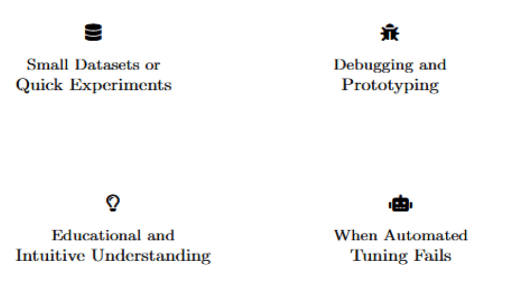
Small datasets or quick experiments Small datasets allow for rapid model training processes. Running multiple manual experiments can be a viable option when working with small datasets.
Debugging and prototyping
When a model fails to perform properly, manual tuning of a single parameter can help diagnose issues. For example, if raising max_depth fails to improve validation accuracy, it suggests that the problem may not be related to model complexity but rather the data quality.
Educational and Intuitive Understanding Manual hyperparameter tuning forces you to grasp the effects of each configuration on model behavior. This is great for learning and debugging. Understanding the bias-variance tradeoff becomes clearer as you observe how model behavior changes through increased complexity or added constraints.
When automated tuning fails
Automated searches often fail to escape suboptimal regions and may become confused by noise. Human intuition can spot patterns within results and choose to experiment with new approaches (for example, “all high values of parameter X perform poorly, so we will try a very low value of X”).
FAQ SECTION
Why manually tune ML parameters instead of using automation? Using manual control methods develops intuition, saves computing resources, and resolves issues faster than black-box search techniques.
What parameters should I tune first in a model? Focus tuning efforts on those hyperparameters that have the greatest impact on your model’s performance:
- When using neural networks, the learning rate is usually the primary hyperparameter to tune. Subsequently, you can tune the number of layers/units, batch size, and regularization strength, which includes L2 and dropout parameters.
- With tree-based models, tree depth, the number of trees (estimators), and the learning rate (for boosted trees) are important.
- For the SVM algorithm, the parameters C and kernel gamma, when using the RBF kernel.
- For k-Nearest Neighbors, the number of neighbors is k.
Can manual tuning improve model accuracy significantly?
A model can benefit from manual tuning, particularly when the initial hyperparameters were poorly chosen. The default settings on many models lead to suboptimal performance for specific problems. Through manual tuning, you can elevate the accuracy levels of your model.
Is manual parameter tuning still relevant today? Absolutely. In the modern AutoML era, practitioners still depend on manual sweeps to meet performance, latency, and regulatory standards.
Conclusion
Data scientists and machine learning engineers must maintain manual hyperparameter tuning as a fundamental skill in their toolbox. Exploring various settings through one-at-a-time tests, manual grid searches, or random searches provides a comprehensive understanding of how key parameters influence the bias-variance trade-off and the model’s performance.
Using best practices like coarse-to-fine searches, clear logging, and thorough validation makes each trial purposeful and reproducible. When running experiments on DigitalOcean GPU Droplets, you have full control over your compute environment—ideal for manually tweaking hyperparameters using frameworks like PyTorch or TensorFlow.
The manual approach lets you identify issues and teach concepts while making informed decisions when resources or time are limited.
For more in-depth tutorials and examples, explore these resources:
Thanks for learning with the DigitalOcean Community. Check out our offerings for compute, storage, networking, and managed databases.
About the author(s)
I am a skilled AI consultant and technical writer with over four years of experience. I have a master’s degree in AI and have written innovative articles that provide developers and researchers with actionable insights. As a thought leader, I specialize in simplifying complex AI concepts through practical content, positioning myself as a trusted voice in the tech community.
With a strong background in data science and over six years of experience, I am passionate about creating in-depth content on technologies. Currently focused on AI, machine learning, and GPU computing, working on topics ranging from deep learning frameworks to optimizing GPU-based workloads.
Still looking for an answer?
This textbox defaults to using Markdown to format your answer.
You can type !ref in this text area to quickly search our full set of tutorials, documentation & marketplace offerings and insert the link!
 This work is licensed under a Creative Commons Attribution-NonCommercial- ShareAlike 4.0 International License.
Become a contributor for community
Get paid to write technical tutorials and select a tech-focused charity to receive a matching donation.

DigitalOcean Documentation
Full documentation for every DigitalOcean product.

Resources for startups and AI-native businesses
The Wave has everything you need to know about building a business, from raising funding to marketing your product.
The developer cloud
Scale up as you grow — whether you're running one virtual machine or ten thousand.

Start building today
From GPU-powered inference and Kubernetes to managed databases and storage, get everything you need to build, scale, and deploy intelligent applications.
