Understanding t-SNE: Dimensionality Reduction Technique

• t-SNE (t-Distributed Stochastic Neighbor Embedding) is a non-linear dimensionality reduction technique used to visualize high-dimensional data in 2D or 3D.
• It works by preserving local relationships. The monopoly of this technique lies in understanding that the data points that are close in high-dimensional space remain close in the low-dimensional projection.
• Ideal for visualizing complex datasets such as images, word embeddings, or genetic data.
• The algorithm converts pairwise similarities between points into probability distributions, then minimizes the difference between these distributions across high- and low-dimensional spaces.
• t-SNE is computationally heavy for large datasets, but optimized or approximate versions (like Barnes-Hut t-SNE or openTSNE) can improve performance.
• Commonly used for data exploration, clustering validation, and feature understanding in machine learning workflows.

SNE aims to embed high-dimensional data into a lower-dimensional space while preserving the neighborhood structure of points.

Let us first understand the intuition behind SNE:

SNE uses a probabilistic approach:

• Each data point defines a probability distribution over all other points.
• Points close to each other in high-dimensional space should also be close in the lower-dimensional embedding.

Step 1: Computing Similarities in High-Dimensional Space

For two points xi and xj​, the similarity is represented as a conditional probability that xj is a neighbor of xi:

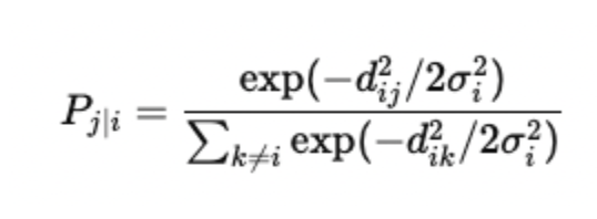
where:

• d 2ij=||xi-xj||2 is the squared Euclidean distance between xi and xj.
• σi controls the width of the Gaussian centered at xi​.

Each σi is determined using binary search so that the perplexity of the conditional distribution equals a user-specified value.

SNE aims to minimize the difference in probability distribution between the higher dimension and the lower dimension.
For each object, i and its neighbor j, we compute a Pi|j which reflects the probability that j is a neighbor of i.

Step 2: The Role of Perplexity

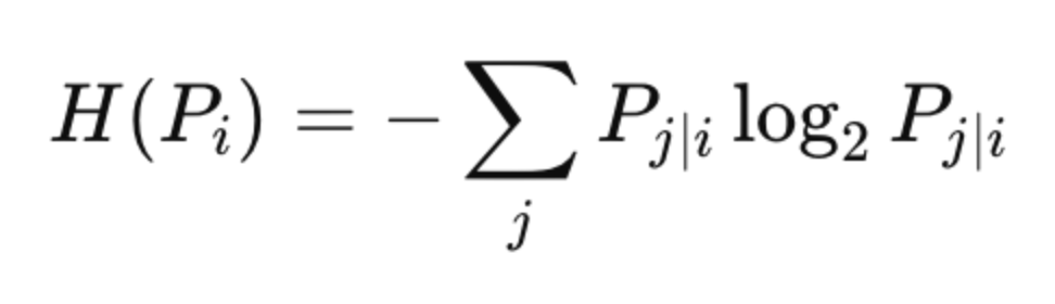
Perplexity reflects the effective number of neighbors for a data point and is defined as:

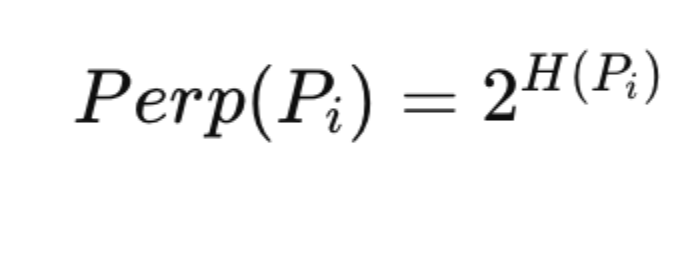
where entropy H(Pi) is given by:

A smaller perplexity emphasizes local structure, while a larger one emphasizes global structure.

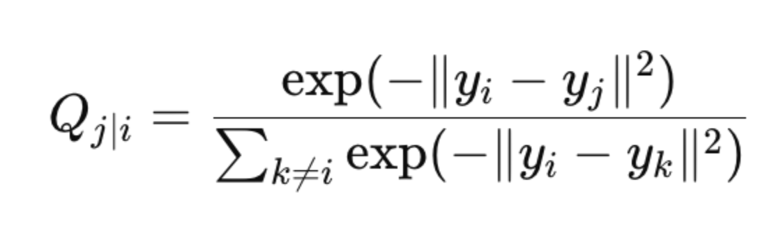
Step 3: Similarities in Low-Dimensional Space

SNE initializes the low-dimensional embeddings yi​ randomly and defines a similar probability distribution in the low-dimensional space:

Step 4: Cost Function

SNE minimizes the mismatch between the high-dimensional and low-dimensional similarity distributions using the Kullback-Leibler (KL) divergence:

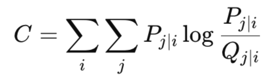
This ensures that points that are close in high-dimensional space remain close in the low-dimensional embedding.

Step 5: Limitations of SNE

Despite its success, SNE suffers from two main issues:

• Asymmetry: Pj∣i≠Pi∣j, leading to inconsistent neighborhood relationships.
• Crowding problem: When projecting from high to low dimensions, there’s not enough “space” to preserve all relative distances and thus leads to overlapping clusters.

To overcome these problems, t-SNE was introduced.

t-SNE, developed by Laurens van der Maaten and Geoffrey Hinton in their paper “Visualizing data using t-SNE”, refines SNE in two major ways:

1. It symmetrizes the similarity matrix.
2. It uses a Student-t distribution with heavy tails in the low-dimensional space to address the crowding problem.

Step 1: Symmetric Similarities

t-SNE defines joint probabilities as:

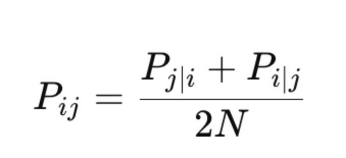
where N is the total number of points.
This makes Pij=Pji leading to a more balanced representation of pairwise similarities.

Step 2: Using Student-t Distribution in Low-Dimensional Space

Instead of using a Gaussian in low dimensions, t-SNE uses a Student-t distribution with one degree of freedom (also known as a Cauchy distribution):

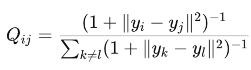
This distribution has heavier tails than a Gaussian, meaning that moderately distant points in high-dimensional space do not get forced too close in the low-dimensional embedding, effectively solving the crowding problem.

Step 3: Cost Function in t-SNE

The KL divergence-based cost function in t-SNE becomes:

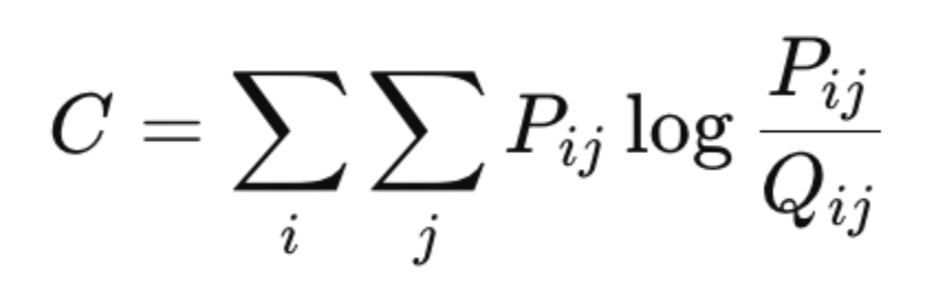
This cost function is minimized using gradient descent, where each iteration adjusts the positions of the points in the low-dimensional map to better align with the high-dimensional similarities.

Step 4: Optimization

The gradient of the cost function is given by:

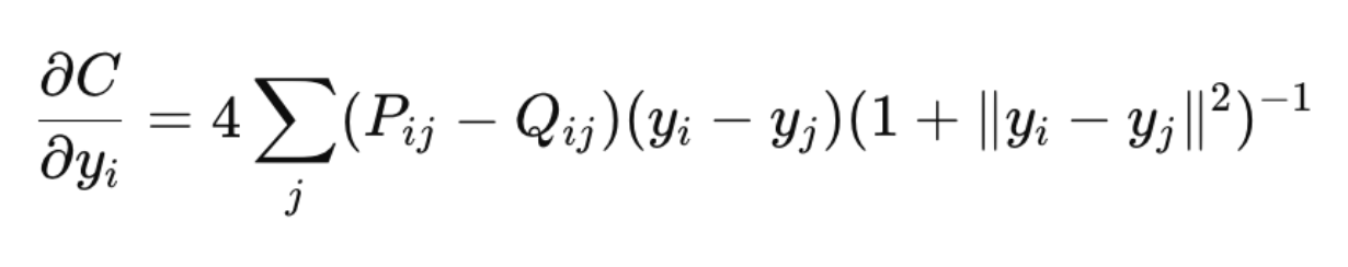
This update rule ensures that similar points attract each other and dissimilar points repel each other.

The perplexity parameter in t-SNE plays a crucial role in determining the granularity of clusters.

• Low perplexity → captures local structures, but may overfit and create too many small clusters.
• High perplexity → captures global structure, but may merge distinct clusters.

In practice, values between 5 and 50 usually yield good results.

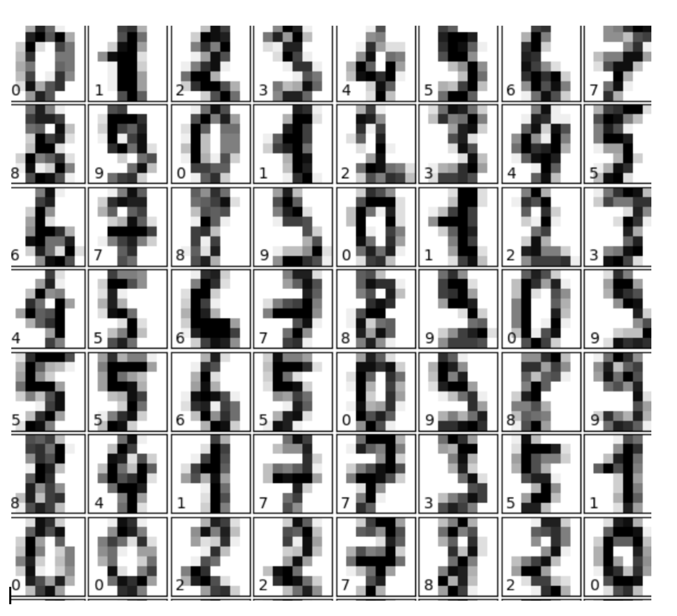
Let’s walk through a practical example using the Digits dataset, which contains images of handwritten digits (0–9). Each image has 64 features (8×8 pixels). We’ll use t-SNE to visualize these high-dimensional data points in 2D space.

# Import required libraries
from sklearn.datasets import load_digits
from sklearn.manifold import TSNE
import matplotlib.pyplot as plt

# Load the dataset
digits = load_digits()
X = digits.data
y = digits.target

# Apply t-SNE to reduce the dimensions to 2D
tsne = TSNE(n_components=2, random_state=42, perplexity=30, learning_rate=200)
X_embedded = tsne.fit_transform(X)

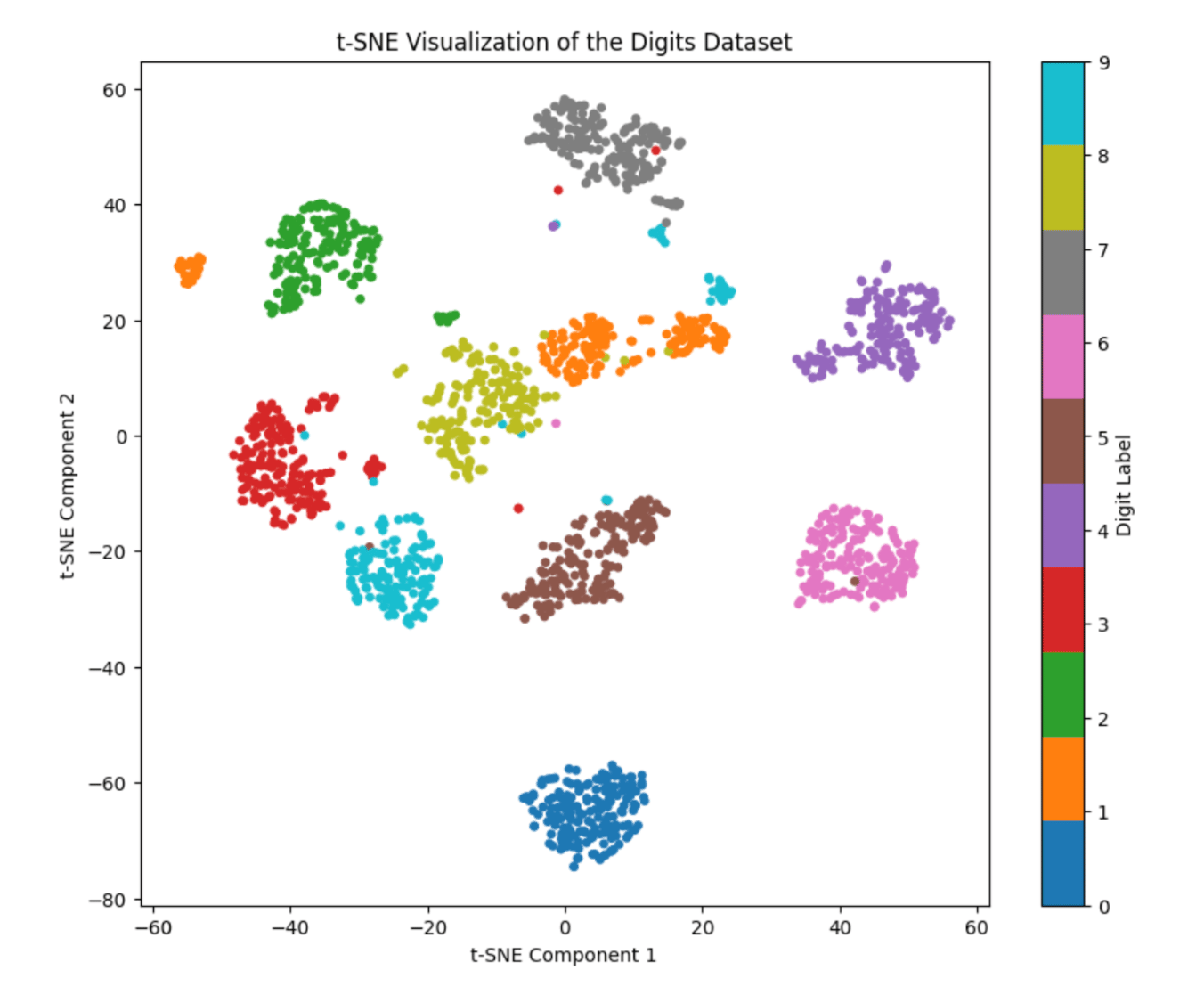
# Visualize the 2D projection
plt.figure(figsize=(10, 8))
scatter = plt.scatter(X_embedded[:, 0], X_embedded[:, 1], c=y, cmap='tab10', s=15)
plt.colorbar(scatter, label="Digit Label")
plt.title("t-SNE Visualization of the Digits Dataset")
plt.xlabel("t-SNE Component 1")
plt.ylabel("t-SNE Component 2")
plt.show()

Here, the load_digits() function loads a dataset of 1,797 handwritten digit samples.

Next, the TSNE() function is used to convert the 64-dimensional data into 2D while preserving local similarities. Perplexity controls how t-SNE balances attention between local and global data structure (typically between 5–50).

The final scatter plot shows similar digits clustered together, for example, all “0”s form one group, “1”s another, and so on.

Despite its impressive performance, t-SNE has a few drawbacks:

• Computationally expensive: Especially for large datasets, since it requires pairwise similarity calculations.
• Non-convex optimization: The algorithm can get stuck in local minima.
• Not scalable: Difficult to handle datasets with millions of points without modifications.

To address these, optimized versions like Barnes-Hut t-SNE and FFT-accelerated t-SNE (FIt-SNE) have been developed to improve scalability and speed.

Q1. What is the main goal of t-SNE?
The main goal of t-SNE is to represent high-dimensional data in a low-dimensional space (typically 2D or 3D) while maintaining the relative similarities between data points.

Q2. How is t-SNE different from PCA?

• PCA is a linear method that focuses on maximizing variance along new axes.
• t-SNE, on the other hand, is non-linear and preserves local structure, making it better for visualizing clusters and complex manifolds.

Q3. What does the “t” in t-SNE stand for?
The “t” stands for Student’s t-distribution, which t-SNE uses in its low-dimensional space to prevent crowding and overlap among clusters.

Q4. What are the key parameters to tune in t-SNE?

• Perplexity: Influences the balance between local and global aspects of the data (usually between 5–50).
• Learning rate: Controls how fast the optimization proceeds (values between 100–1000 often work well).
• n_iter: Number of optimization iterations (default is 1000, but 2000+ may yield better results).

Q5. When should I use t-SNE?
Use t-SNE for exploratory data analysis, particularly when you want to visualize hidden patterns, separations, or clusters in high-dimensional datasets, such as image embeddings, NLP features, or genetic data.

Q6. Can t-SNE be used for feature reduction before model training?
Not ideally. t-SNE is best suited for visualization, not for feature reduction in predictive modeling, since it does not preserve global distances or scales consistently.

Q7. What are some alternatives to t-SNE?
You can try UMAP, PCA, or Isomap. UMAP, in particular, offers similar results to t-SNE but runs faster and scales better for larger datasets.

t-SNE has reformed the way we visualize and understand high-dimensional data. By using a Student-t distribution and symmetric probability measures, it produces beautiful, interpretable 2D or 3D embeddings that capture both local and global relationships.

However, due to its computational intensity, researchers often use optimized versions like Barnes-Hut t-SNE or Fit-SNE for large-scale applications.

For those looking to go beyond simple visualization, exploring parametric t-SNE and deep t-SNE opens up exciting possibilities. These approaches combine the power of neural networks with t-SNE’s ability to uncover meaningful low-dimensional representations, making it easier to scale and apply to new data.

• Principal Component Analysis (PCA) in Machine Learning
• Understanding One-Hot Encoding in Machine Learning
• Intro to optimization in deep learning: Gradient Descent
• A Practical Guide to Random Forests in Machine Learning
• Linear Probability Model: Definition, Examples & Limitations