AI Technical Writer
 in Machine Learning")
What if there is a simple way to achieve faster training using simple machine learning algorithms? That’s exactly what Principal Component Analysis (PCA) helps to achieve. PCA is a powerful technique that helps to simplify large and complex datasets by reducing their dimensionality and also preserving the important information as much as possible.
By transforming correlated features into a smaller set of uncorrelated components, PCA allows models to train faster, perform better, and avoid issues like overfitting.
PCA was introduced by Karl Pearson, a British mathematician, in 1901 as a statistical method to analyze data variation and relationships. Decades later, Harold Hotelling expanded on Pearson’s work in the 1930s, formalizing the mathematical foundation that is still used today. With the rise of digital computation and data-driven research, PCA naturally found its place in machine learning, where it became an essential preprocessing step for feature extraction, noise reduction, and data visualization.
In this article, we will break down what PCA is, why it is important, and explore how to implement it in Python with practical examples for real-world applications.
Key Takeaways
- PCA simplifies complex datasets by reducing the number of features while keeping most of the important information.
- It helps speed up training and reduce computational costs by working with fewer dimensions.
- PCA is an unsupervised method, meaning it doesn’t need labeled data to find patterns.
- It creates new features called principal components, which capture the maximum variance in the data.
- Scaling features before applying PCA is important to ensure that no single variable dominates the analysis.
- PCA is useful for data visualization, noise reduction, and feature extraction in machine learning. However, it can make features less interpretable, since the new components are combinations of the original ones.
Before we dive into understanding PCA, let us first understand why it is needed.
As we understood, PCA helps to simplify datasets by reducing the number of features while preserving as much relevant information as possible. This makes models faster to train and easier to interpret. Further, PCA helps to create new features, also known as principal components, which are uncorrelated and helps to capture maximum variance in the data.
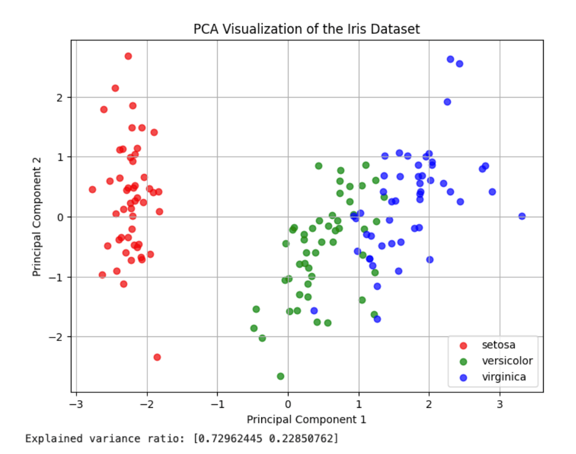
By focusing only on the most significant components, PCA filters out less important variations that usually represent noise. It also allows high-dimensional data to be represented in 2D or 3D plots, helping to uncover patterns, trends, and clusters visually.
What is Principal Component Analysis (PCA)?
Imagine a dataset with more than 100 features like age, height, weight, BMI, hours of sleep, and so on. Now, if you are building a machine learning model, some of these features might carry weightage or the right information for the model, while others do not matter much and are just noise. Looking at all these features is overwhelming for both humans and machines.
PCA is a dimensionality reduction technique or feature reduction technique that simplifies complex datasets by reducing the number of features. It does this by creating new features, called principal components, which are combinations of the original features and capture the most important patterns in the data.
For instance, a dataset with 100 features can often be represented effectively with fewer dimensions using PCA. This not only reduces computational complexity but also removes noise and redundant information, leading to faster training of machine learning models, less data to process, and often improved model performance.
How PCA Works: Step-by-Step Explanation
Example Dataset: Student Marks
Let’s say we have marks of 6 students in 3 subjects:
| Student | Math | Science | English |
|---|---|---|---|
| A | 85 | 80 | 78 |
| B | 90 | 85 | 88 |
| C | 78 | 70 | 72 |
| D | 92 | 88 | 85 |
| E | 70 | 65 | 68 |
| F | 88 | 82 | 80 |
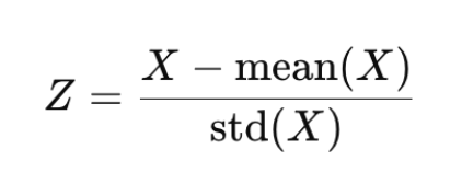
Step 1: Standardize the Data
Each subject may have different scales or ranges. Standardization ensures all features are in the same scale and contribute equally by making them mean-centered and unit-scaled.
import numpy as np
import pandas as pd
import matplotlib.pyplot as plt
from sklearn.preprocessing import StandardScaler
# Step 1: Create dataset
data = {
    'Math': [85, 90, 78, 92, 70, 88],
    'Science': [80, 85, 70, 88, 65, 82],
    'English': [78, 88, 72, 85, 68, 80]
}
df = pd.DataFrame(data)
print("Original Data:\n", df)
# Step 2: Standardize
scaler = StandardScaler()
scaled_data = scaler.fit_transform(df)
df_scaled = pd.DataFrame(scaled_data, columns=df.columns)
print("\nStandardized Data:\n", df_scaled)
Original Data:
    Math  Science  English

0    85       80       78

1    90       85       88

2    78       70       72

3    92       88       85

4    70       65       68

5    88       82       80
Standardized Data:
        Math   Science   English

0  0.153008  0.203785 \-0.072232

1  0.808755  0.815139  1.372399

2 \-0.765039 \-1.018924 \-0.939010

3  1.071054  1.181952  0.939010

4 \-1.814235 \-1.630278 \-1.516862

5  0.546456  0.448327  0.216695
Here we have used StandardScaler() to make each feature mean = 0 and std = 1, and hence the features are comparable.
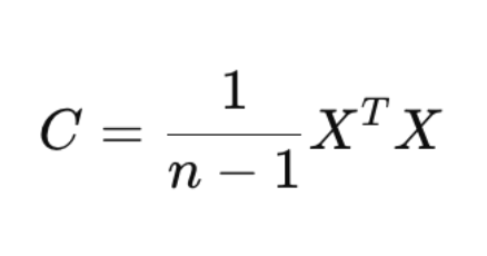
Step 2: Compute the Covariance Matrix
Covariance measures how two variables change together. If Math and Science have high positive covariance → students scoring high in Math also score high in Science.
PCA uses covariance to find correlated patterns and reduce redundancy.
# Step 3: Compute Covariance Matrix
cov_matrix = np.cov(df_scaled.T)
print("\nCovariance Matrix:\n", cov_matrix)
Covariance Matrix:
[[1.2 1.18771556 1.13866982]
[1.18771556 1.2 1.14813529]
[1.13866982 1.14813529 1.2 ]]
We transpose the matrix (.T) because covariance is computed between features (columns). A high value means features vary together strongly.
Step 3: Calculate Eigenvalues and Eigenvectors
- Eigenvectors → directions (axes) of maximum variance.
- Eigenvalues → amount of variance in those directions.
PCA sorts eigenvectors by their eigenvalues to find the most informative directions.
# Step 4: Compute Eigenvalues and Eigenvectors
eigenvalues, eigenvectors = np.linalg.eig(cov_matrix)

print("\nEigenvalues:\n", eigenvalues)
print("\nEigenvectors:\n", eigenvectors)
Eigenvalues:
[3.51647796 0.01177375 0.07174828]
Eigenvectors:
[[-0.5790409 -0.66755048 -0.46806837]
[-0.58058703 0.74067789 -0.33810496]
[-0.57239002 -0.07597782 0.81645394]]
Each eigenvector corresponds to a new axis (principal component). The eigenvalue tells how much variance that axis captures.
Step 4: Select Principal Components
We’ll sort eigenvalues in descending order and pick the top ones that explain the most variance.
# Step 5: Sort and Select Principal Components
explained_variance_ratio = eigenvalues / sum(eigenvalues)
print("\nExplained Variance Ratio:\n", explained_variance_ratio)

# Sort eigenvectors based on eigenvalues
sorted_index = np.argsort(eigenvalues)[::-1]
sorted_eigenvectors = eigenvectors[:, sorted_index]

# Choose top 2 components
n_components = 2
eigenvector_subset = sorted_eigenvectors[:, 0:n_components]
Explained Variance Ratio:
[0.97679943 0.00327049 0.01993008]
We see how much variance each component captures (ratio). Typically, we choose the smallest number of components that explain ~95% of the variance.
Step 5: Transform the Data
We now project the original (standardized) data onto the new axes (principal components).
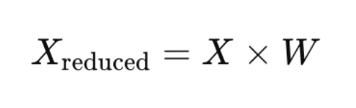
W = matrix of selected eigenvectors.
# Step 6: Transform the data
pca_data = np.dot(df_scaled, eigenvector_subset)

df_pca = pd.DataFrame(pca_data, columns=['PC1', 'PC2'])
print("\nTransformed Data (PCA Results):\n", df_pca)
Transformed Data (PCA Results):
PC1 PC2
0 -0.165568 -0.199492
1 -1.727109 0.466345
2 1.572042 -0.064064
3 -1.843890 -0.134292
4 2.865271 0.161943
5 -0.700747 -0.230439
The dataset is now reduced from 3D (Math, Science, English) → 2D (PC1, PC2).
These components capture most of the original variance.
Step 6: Visualize the Results
# Step 7: Plot the PCA results
plt.figure(figsize=(6, 5))
plt.scatter(df_pca['PC1'], df_pca['PC2'], color='blue')
plt.title('PCA Result: Student Marks Projected onto 2 Principal Components')
plt.xlabel('Principal Component 1')
plt.ylabel('Principal Component 2')
for i, student in enumerate(['A', 'B', 'C', 'D', 'E', 'F']):
    plt.text(df_pca['PC1'][i]+0.02, df_pca['PC2'][i]+0.02, student)
plt.grid(True)
plt.show()
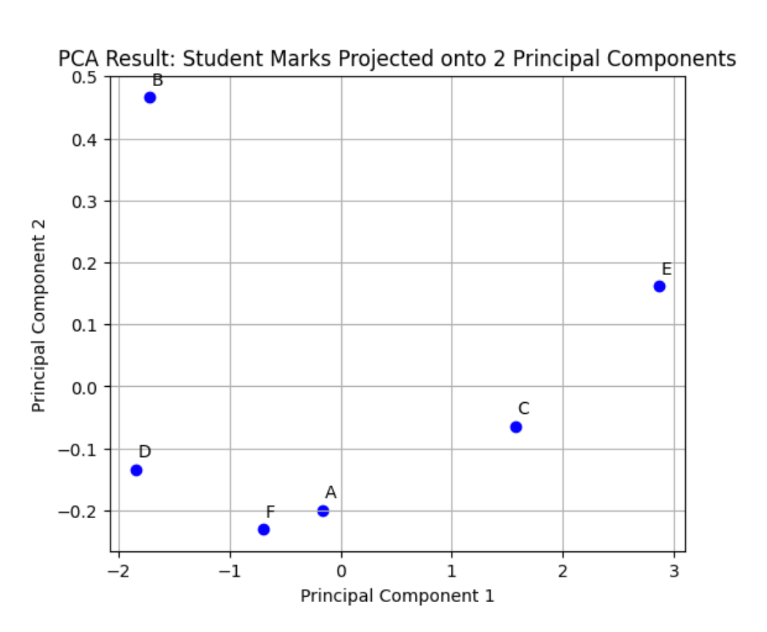
Each dot represents a student. Students close together have similar mark patterns across subjects. Thus, we’ve simplified our dataset to 2D while preserving the essence of the original 3D data.
Using sklearn.decomposition.PCA
You can perform PCA in one line with scikit-learn:
from sklearn.decomposition import PCA

pca = PCA(n_components=2)
principal_components = pca.fit_transform(df_scaled)

print("\nExplained Variance Ratio (Sklearn):", pca.explained_variance_ratio_)
print("\nPCA Components:\n", pca.components_)
Explained Variance Ratio (Sklearn): [0.97679943 0.01993008]
PCA Components:
[[ 0.5790409 0.58058703 0.57239002]
[-0.46806837 -0.33810496 0.81645394]]
The explained variance ratio tells us how much information (variance) each principal component captures from the original dataset.
For example:
- PC1 = 0.85 → captures 85% of total variance
- PC2 = 0.10 → captures 10%
- PC3 = 0.05 → captures 5%
If PC1 + PC2 ≈ 0.95 (or 95%), we can safely reduce 3D → 2D with minimal information loss.
Each principal component is a linear combination of original features. The explained variance ratio tells you how much of the original dataset’s information is preserved.
PCA with other dimensionality reduction techniques
| Technique | Type | Preserves Global Structure | Non-linear Capability | Typical Use Case | Explanation |
|---|---|---|---|---|---|
| PCA (Principal Component Analysis) | Linear (unsupervised) | Yes | No | Feature extraction, noise reduction, and visualization | PCA identifies directions (principal components) that capture the maximum variance in data. It works well when relationships between features are linear and helps simplify datasets for training or visualization. |
| t-SNE (t-Distributed Stochastic Neighbor Embedding) | Non-linear (unsupervised) | No | Yes | Visualizing high-dimensional data, such as word embeddings or image features | t-SNE focuses on preserving local relationships rather than overall structure. It’s great for showing clusters in data, but not ideal for feature extraction because it can distort global distances. |
| LDA (Linear Discriminant Analysis) | Linear (supervised) | Yes | No | Classification and dimensionality reduction for labeled data | LDA uses class labels to find axes that best separate different categories. It reduces dimensions while maintaining class separability, making it useful in classification tasks like face recognition or text categorization. |
Loading in PCA
In PCA, loadings represent how much each original feature adds weightage to each principal component.
They show the correlation or weight between the original features (like Math, Science, English) and the new PCA axes (like PC1, PC2).
In simple terms:
- A high positive loading means that the feature contributes strongly and positively to that principal component.
- A high negative loading means that the feature contributes strongly but in the opposite direction.
- Small or near-zero loadings mean that the feature doesn’t influence that component much.
import numpy as np
import pandas as pd
from sklearn.preprocessing import StandardScaler
from sklearn.decomposition import PCA

# Dataset
data = {
    'Math': [85, 90, 78, 92, 70, 88],
    'Science': [80, 85, 70, 88, 65, 82],
    'English': [78, 88, 72, 85, 68, 80]
}

df = pd.DataFrame(data)

# Step 1: Standardize the data
scaler = StandardScaler()
df_scaled = scaler.fit_transform(df)

# Step 2: Apply PCA
pca = PCA(n_components=3)
pca.fit(df_scaled)

# Step 3: Extract loadings
loadings = pca.components_.T * np.sqrt(pca.explained_variance_)

# Convert to DataFrame for readability
loading_df = pd.DataFrame(
    loadings,
    columns=['PC1', 'PC2', 'PC3'],
    index=['Math', 'Science', 'English']
)

print("PCA Loadings:\n")
print(loading_df.round(3))
pca.components_gives eigenvectors — directions of each principal component.pca.explained_variance_gives eigenvalues — the variance captured by each component.- Multiplying
components_.T * sqrt(explained_variance_)gives the loadings matrix.
Each cell shows how much a feature contributes to a component.
Common PCA Challenges
While PCA is a powerful tool for simplifying data and building a less complex model, it’s not without its limitations. Below are some common challenges you might face when applying PCA in practice:
- Loss of Interpretability: After transformation, the new principal components are combinations of original features, making it hard to understand what each component represents. Thus making the model a black box model to some extent.
- Assumes Linearity: PCA works best when relationships between variables are linear. It may not perform well on complex, non-linear datasets.
- Sensitive to Feature Scaling: If features are not standardized properly, PCA may give more importance to features with larger numerical ranges.
- Choosing the Number of Components: Deciding how many principal components to keep can be tricky. Too few may lose information, while too many may not simplify the data effectively.
- Outlier Sensitivity: Outliers can disproportionately influence the direction of principal components, leading to misleading results.
It is best to use PCA when you have a dataset that has too many correlated features. Further if there is a need to speed up training without losing accuracy.
FAQ’s
-
Q1. What is PCA used for in machine learning? PCA (Principal Component Analysis) is mainly used for dimensionality reduction, data visualization, and feature extraction. It helps simplify complex datasets by reducing the number of input variables while retaining most of the important information. For example, in machine learning, PCA can make models train faster, reduce overfitting, and help visualize high-dimensional data (like 50 features) in 2D or 3D plots.
-
Q2. Is PCA supervised or unsupervised? PCA is an unsupervised learning technique. This means it doesn’t use labels or target variables during the process. Instead, it looks at the structure of the data itself, identifying the directions (principal components) where the data varies the most. These directions help summarize and simplify the dataset without any prior knowledge of the output classes.
-
Q3. What is the main purpose of PCA? The main purpose of PCA is to capture the maximum variance in the data using fewer features. It achieves this by transforming the original correlated features into a smaller set of new, uncorrelated variables called principal components. These components retain the most significant patterns in the data, allowing for easier visualization, faster training, and improved model performance on high-dimensional datasets.
-
Q4. How does PCA differ from t-SNE? While both PCA and t-SNE are used for dimensionality reduction, they work differently:
-
PCA is a linear technique that identifies straight-line relationships in data. It is primarily used to simplify features while preserving structure. It’s fast, interpretable, and works well for large datasets.
-
t-SNE (t-distributed Stochastic Neighbor Embedding) is a non-linear technique that focuses on visualizing data in 2D or 3D by preserving local relationships between points. It’s ideal for exploring clusters or patterns, but is computationally heavier and not suitable for feature extraction in model training.
-
Q5. How does PCA work? PCA works by transforming your original dataset into a new set of variables called principal components. These components are ordered so that the first few capture most of the variation in the data. It does this using a mathematical process called eigenvalue decomposition or singular value decomposition (SVD), which identifies the directions (axes) where the data varies the most.
-
Q6. When should I use PCA? You should use PCA when your dataset has many correlated features, making it difficult to visualize or train machine learning models efficiently. It’s especially useful before applying algorithms like logistic regression, k-means clustering, or neural networks, as it helps reduce noise, remove redundancy, and improve model performance.
-
Q7. How do you decide how many principal components to keep? You can decide based on the explained variance ratio. Most people choose the number of components that capture around 95%–99% of the total variance. This ensures you’re keeping most of the meaningful information while still simplifying your dataset.
-
Q8. What’s the difference between PCA and Feature Selection? Feature selection chooses a subset of the original features, while PCA creates new features (components) that are combinations of the original ones. In other words, PCA transforms the data, whereas feature selection filters it.
-
Q9. Do we need to scale data before applying PCA? Yes. PCA is sensitive to the scale of features because it relies on variance. If one feature has a much larger range than others, it can dominate the principal components. Therefore, it’s best to standardize or normalize your data before applying PCA.
-
Q10. Can PCA be used for image processing? PCA is widely used in image compression and facial recognition. It helps reduce the number of pixels (features) while preserving the essential visual patterns. This makes image storage and processing much faster without a major loss in quality.
Conclusion
In this article, we discussed Principal Component Analysis (PCA), a powerful and widely used technique for simplifying complex datasets. PCA helps retain most of the important information by transforming correlated features into a smaller set of uncorrelated components. It also helps reduce dimensionality, improve model performance, and make data visualization easier.
Through steps like standardization, covariance calculation, and eigen decomposition, PCA identifies the directions of maximum variance in the data. The explained variance ratio helps determine how much information each component preserves, while loadings reveal which original features contribute most to each principal component.
Although PCA is efficient and interpretable for linear relationships, it comes with its limitations, such as sensitivity to outliers, the need for scaling, and challenges in interpreting transformed features. Overall, PCA remains a fundamental tool in any data scientist’s toolkit, offering a balance between simplicity, interpretability, and effectiveness for exploratory analysis, visualization, and feature extraction.
Thanks for learning with the DigitalOcean Community. Check out our offerings for compute, storage, networking, and managed databases.
About the author
With a strong background in data science and over six years of experience, I am passionate about creating in-depth content on technologies. Currently focused on AI, machine learning, and GPU computing, working on topics ranging from deep learning frameworks to optimizing GPU-based workloads.
Still looking for an answer?
This textbox defaults to using Markdown to format your answer.
You can type !ref in this text area to quickly search our full set of tutorials, documentation & marketplace offerings and insert the link!
 This work is licensed under a Creative Commons Attribution-NonCommercial- ShareAlike 4.0 International License.
Become a contributor for community
Get paid to write technical tutorials and select a tech-focused charity to receive a matching donation.

DigitalOcean Documentation
Full documentation for every DigitalOcean product.

Resources for startups and AI-native businesses
The Wave has everything you need to know about building a business, from raising funding to marketing your product.
The developer cloud
Scale up as you grow — whether you're running one virtual machine or ten thousand.

Start building today
From GPU-powered inference and Kubernetes to managed databases and storage, get everything you need to build, scale, and deploy intelligent applications.
