By Adrien Payong and Shaoni Mukherjee

Introduction
Hidden Markov Models (HMMs) are probabilistic models in machine learning that capture patterns in sequential data. An HMM posits an underlying sequence of hidden states that transition over time. In addition, each state generates an observable output according to specific emission probabilities.
These models are powerful for inferring hidden structures in dynamic systems where the unobservable causes must be inferred from observable effects. HMMs handle uncertainty and temporal dependencies in sequence data. This guide will provide an overview of HMM theory (transition and emission probability matrices (EM)), key algorithms, implementing HMMs in Python, and modern alternatives for sequence modeling.
Key Takeaways
- HMMs model hidden causes behind observable sequences: They assume an underlying (latent) Markov process that is not observable directly. But it is instead related to the observations through emission probabilities. This makes them suitable for problems where you can only observe effects, not the true underlying states.
- Three core problems define HMM usage: Evaluation (calculating the observation likelihood using the Forward algorithm), Decoding (recovering the most likely hidden sequence with Viterbi), and Learning (learning the model parameters with Baum–Welch or EM).
- Interpretability is a major strength: The parameters of the model (initial state probabilities, transition matrix, and emission probabilities) all have a probabilistic meaning, making HMMs more interpretable and intuitive than deep neural networks.
- HMMs remain practical for smaller or structured datasets: HMMs can be effective when there is limited data or when domain knowledge defines transitions. This includes speech recognition, genomics, and financial market regime detection.
- Modern deep models extend their spirit: Deep models like RNNs, Transformers, and hybrid HMM-NN models generally outperform HMMs in many large-scale applications. However, they all aim at learning temporal dependencies and capturing uncertainty over time, reflecting the original motivation of HMMs.
What is a Hidden Markov Model?
Hidden Markov Models are probabilistic models for sequence data where an underlying hidden (latent) Markov process generates observable outputs. In an HMM, each time step has a hidden state that evolves with Markovian transitions. There is also an emission probability that produces an observable symbol or feature given each hidden state.
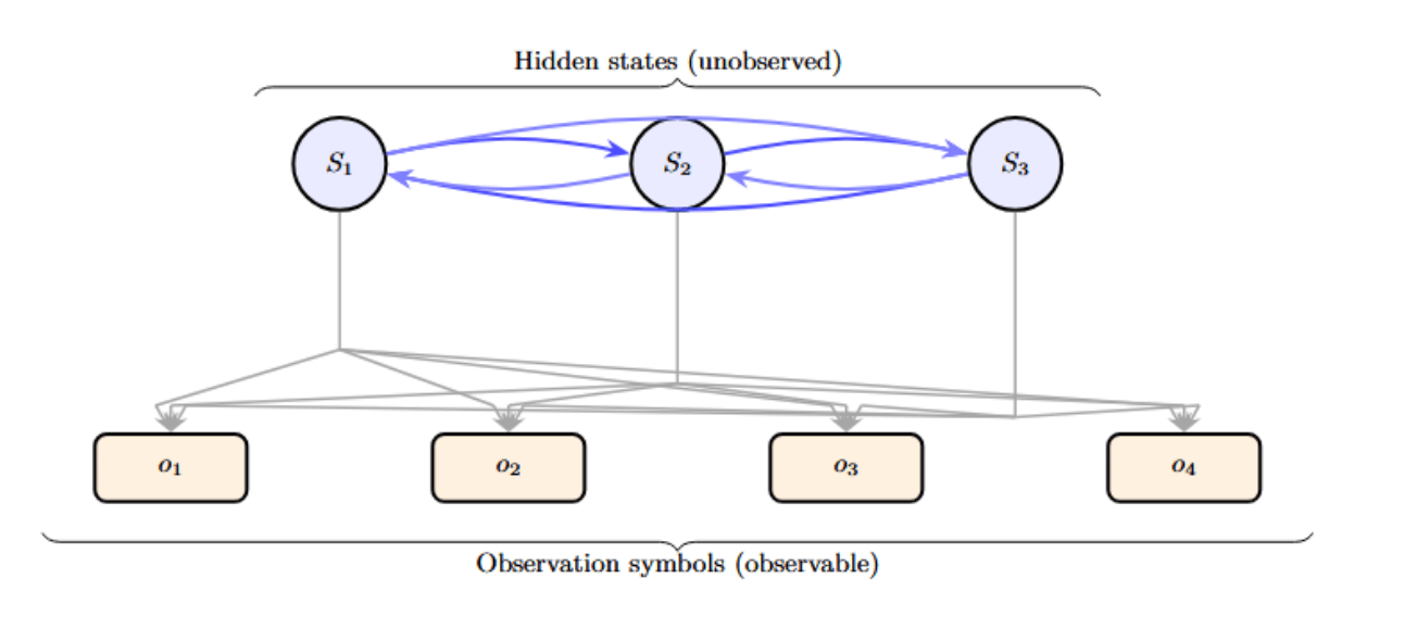
The diagram below shows a basic HMM with three hidden states (circles) and four possible observations (the boxes). Arrows connecting the states indicate the transition probabilities between hidden states. Arrows pointing from a state to an observation indicate the emission probabilities of each of the observable symbols. An HMM learns the transition and emission matrices, thereby modeling how hidden states produce observed sequences in a stochastic process.
Markov Chains vs. Hidden Markov Models
A Markov chain is a simpler model. It has states and transition probabilities. However, all of the states are directly observable. If you were modeling weather with a Markov chain, you could label your states “Sunny”, “Rainy”, etc. In that case, you would directly observe the weather on a given day. The chain then tells you the probability of transitioning from one state today to another state tomorrow.
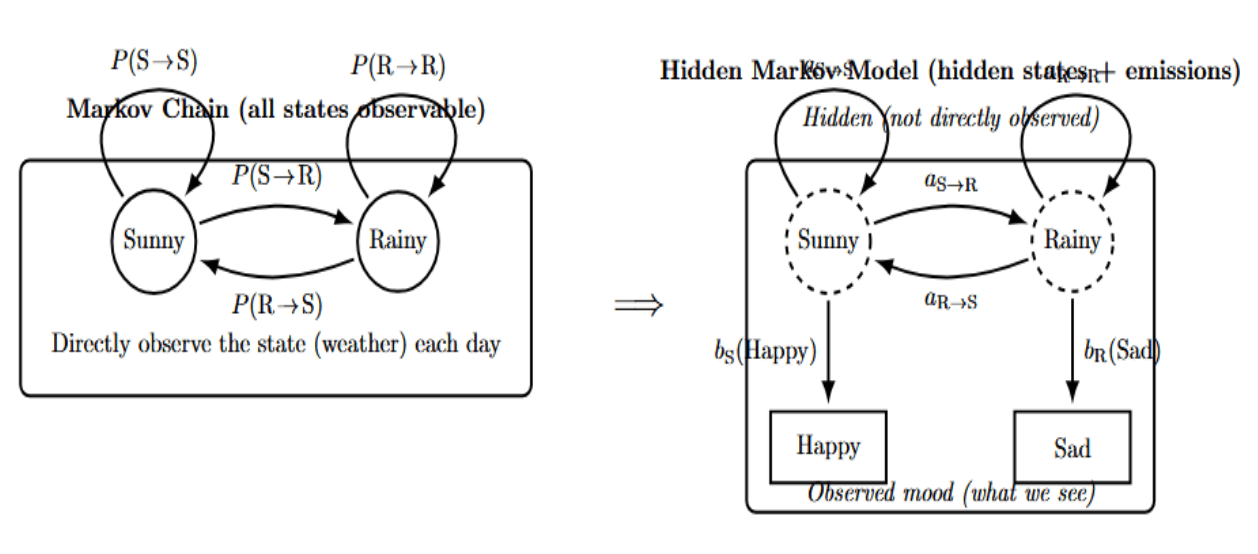
In a Hidden Markov Model, the states are not directly observable. Instead, each state probabilistically produces an observation. In the weather example, you (living in a different city) don’t know what the actual weather is in your friend’s city (hidden state), but you get a phone call about how your friend is feeling (observation). You receive daily updates like “friend is happy” or “friend is sad” that provide insight into the weather conditions in your friend’s city. The hidden weather state affects the observed friend’s mood, but you never directly observe the weather.
Key Components of a Hidden Markov Model — Diagram Overview
Think of this as a quick legend for the HMM diagram: it labels the hidden states and observed symbols and the probability tables (π, A, B) that respectively specify the start, drive transitions, and generate emissions.
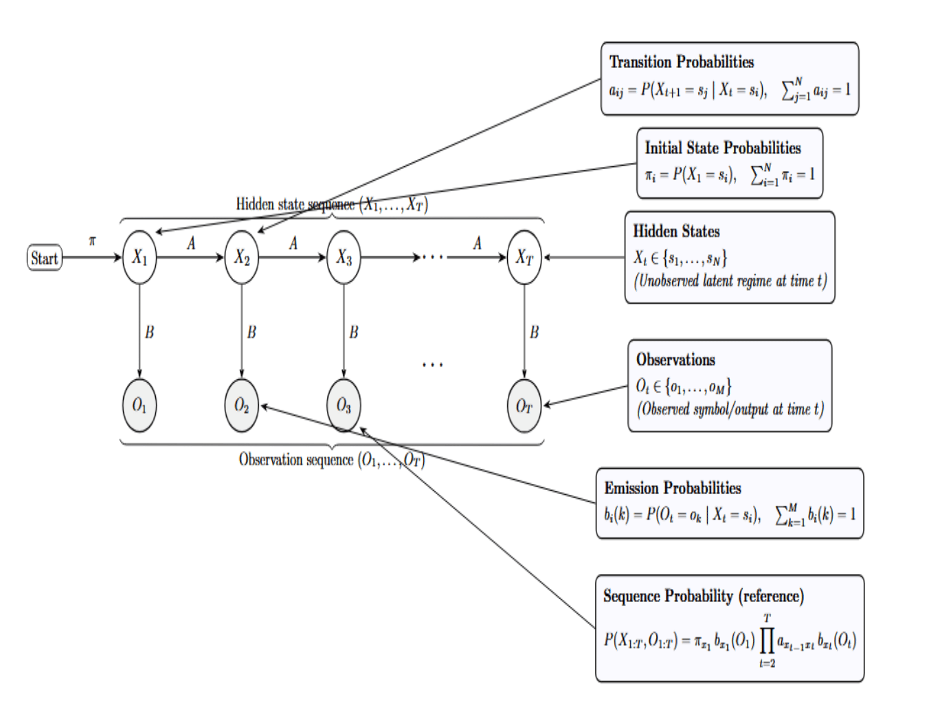
- Hidden States: At each time step t, the system is in exactly one latent class s_i . The notation indicates that the hidden process is categorical, with N possible regimes. X_t itself is never directly observed; you infer it from the data.
- Observations: There is a single observable symbol (or measurement) from a finite alphabet at each time step. This conveys that the data stream we see is discrete in this setting. In practice, O_t is related to X_t: different hidden states generate different patterns of observations.
- Initial State Probabilities: The row vector π describes your a priori belief about where the sequence starts. Each πi is the probability that the very first hidden state is s_i. The normalization reminds you that this is a valid probability distribution.
- Transition Probabilities: The matrix A=[aij] captures state dynamics: from state i, which next states j are likely? The row-stochastic constraint (rows sum to one) ensures each row is a proper conditional distribution. The conditioning on X_t formalizes the first-order Markov property: The future state depends only on the present, and not on the sequence that led to it.
- Emission Probabilities: For each hidden state s_i, the row bi(⋅) is a categorical distribution over the observation symbols. If b_i(k) is high, then state s_i frequently emits the observation symbol o_k. This conditional structure links the unseen process to the observed data.
- Sequence Factorization (Generative Story): This product form is essentially the complete generative story: first select a starting state with π. Then emit the first observation with B, and for each time step, select a new state with A and emit an observation with B.
Example: Weather and Mood HMM
To better understand these components, let’s build a toy HMM example. We will consider the example from above: your friend’s mood depends on the weather in their city. You want to model the system, which involves the following:
- Hidden states: The weather in your friend’s city each day. Let’s assume that we have two states for simplicity: Sunny and Rainy.
- Observations: Your friend’s mood each day, which can be either Happy or Sad.
- State transition probabilities: The probability of the weather changing from one day to another.
- Emission probabilities: How the weather influences the mood.
Let’s suppose that we have the following definition for the model:
# HMM Example: Weather and Friend's Mood
States (hidden): [Sunny, Rainy]
Observations: [Happy, Sad]

Transition probability matrix (A):
          to Sunny   to Rainy
Sunny        0.8        0.2
Rainy        0.4        0.6

Emission probability matrix (B):
             Happy     Sad
Sunny         0.9      0.1
Rainy         0.2      0.8

Initial state distribution (π):
Sunny: 0.5,  Rainy: 0.5
Let’s interpret this HMM:
- If today is sunny, the chance of tomorrow being sunny is 80% (rainy is 20%). If today is rainy, the chance it will be sunny tomorrow is 40% (and rainy 60%). (Rows of the transition matrix add to 1, as they should.)
- On a Sunny day, the probability that your friend is happy is 0.9 (90%) and Sad is 0.1. On a rainy day, there is only a 20% chance they are happy (they may not like rain!) and an 80% chance they are sad. (Rows of the emission matrix also sum to 1.)
- On day 1, we have no information, so we assign an equal probability of being Sunny or Rainy (we could change this if we had information beforehand).
Using this HMM, we can answer different types of questions:
- Sequence likelihood (Evaluation): What is the probability of a given sequence of moods? E.g., what is the probability that, over three days, your moods were [Happy, Happy, Sad]? We need to sum over all possible sequences of weather (that could have caused that mood sequence). The forward algorithm allows this computation in a single pass.
- Most likely hidden sequence (Decoding): Suppose we have an observation sequence of moods, and want to infer the weather sequence. E.g., given [Happy, Sad, Happy], was the weather sequence [Sunny, Rainy, Sunny], [Sunny, Sunny, Sunny], or something else? The Viterbi algorithm computes the best state sequence that explains the observations.
- Learning from data (Training): If we have many observed sequences (and possibly partial state info), how do we learn the HMM parameters (A, B, pi)? The Baum-Welch algorithm (expectation-maximization approach) computes probabilities that maximize the likelihood of the data.
We will get into the details of the Viterbi and Baum-Welch algorithms in the next section. They are the two main algorithms for actually using HMMs in practice. For completeness, though, here is a short review of the three main problems that can be solved by an HMM:
- Evaluation (Likelihood of observations): Given the model, we compute the probability of an observation sequence. (Solved by the Forward algorithm, or Forward-Backward algorithm if we also compute the backward probabilities.)
- Decoding (Most likely state path): Find the single best state sequence that could have generated the observations. (Solved by the Viterbi algorithm; A dynamic programming version of argmax path.)
- Learning (Parameter estimation): Given some observed sequences (and perhaps some initial parameter guesses), find model parameters that maximize the probability of the observed sequences. (Solved by the Baum-Welch algorithm. It uses the forward-backward algorithm internally.)
The Viterbi Algorithm: Decoding HMMs
The Viterbi algorithm is a dynamic programming algorithm that computes the most likely sequence of hidden states for a given observation sequence using an HMM model. This is the solution to the decoding problem. Viterbi decoding is important in applications where we have a sequence of data(such as speech recognition or POS tagging) and we are interested in the most likely explanation (state sequence) of this data.
How it works: Viterbi leverages dynamic programming to avoid brute-force enumeration of all possible paths. At each step, the algorithm efficiently searches through all possibilities by keeping only the highest-probability path to each state at each time step, and incrementally building them. The Viterbi algorithm, therefore, keeps a DP table viterbi[t][i] = probability of the most likely path ending in state i at time t (this is usually stored as a log-probability to prevent underflow). It also uses backpointers to recover the actual sequence at the end.
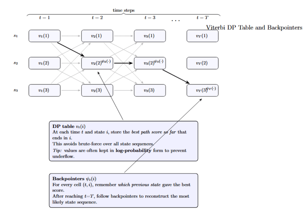
Viterbi DP Table — Simple View
- The grid shows time steps left to right and possible states top to bottom.
- Faint arrows indicate that the algorithm will explore all paths that go from one time step to the next.
- The bolded path will eventually indicate the single most probable path through the states.
- The value of each cell is the best score so far for a path ending in that state at that time.
- Backpointers (small annotations) keep track of which state led to each best score, so that we can trace the path back at the end.
At t=1, it initializes using the initial distribution and emission probabilities:
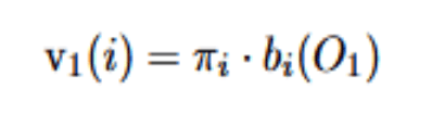
The above is the probability of starting in state i and emitting the first observation O_1.
Then, for each subsequent time t and each state j, it computes:
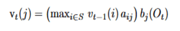
At time t, we want the best score for ending in state j. We get it in three simple moves:
- Look back one step. For each possible previous state i, take the best score in i at time t−1, multiply by the probability of transitioning from i to j. This yields a candidate score for ending up in j coming from i.
- Choose the best route. Pick the largest of those candidate scores. This is the best way to have arrived in J before considering the new observation.
- Check how well j explains the data at time t. Multiply that best route by how likely state j would be to produce the current observation. This “fits” the new data and gives the final score for being in j at time t.
The Baum-Welch Algorithm: Training HMMs
Baum-Welch can be used to train an HMM when you have data, but don’t know the model parameters. It is an Expectation-Maximization (EM) algorithm specialized to HMMs (named after Leonard Baum, who, with other co-authors, published it). Baum-Welch will estimate the transition probabilities A and emission probabilities B (and sometimes initial pi) that most likely generated the observed sequences.
When to use: Let’s say we have a set of observation sequences. We hypothesize that observations are generated by an HMM with some number of states. However, we do not know the specific transition or emission probabilities. Baum-Welch can be used to find a (locally) optimal set of probabilities that maximizes the probability of our data.
How the Baum-Welch Algorithm Works
Baum-Welch iteratively alternates between expecting and maximizing – it’s essentially an EM algorithm:
Expectation (E-step)
Given the current estimate of the model parameters, compute the “expected” number of transitions and emissions in the data. This is done via the forward-backward procedure. Let’s consider the following diagram:
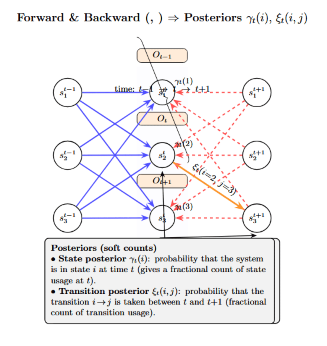
The forward algorithm computes partial probabilities (generally known as α values) for each possible state at each time, given the observations up to that point (represented by the blue lines pointing from earlier times to the current time in the picture).
The backward algorithm computes partial probabilities (β values) from that time forward. This summarizes the likelihood of future observations given each state at the current time. It is visualized by the red-dashed lines moving from the current time to the future states in the image.
Maximization (M-step)
The maximization step re-estimates the model parameters so they fit the data “best” (using the soft counts, i.e., expected sufficient statistics computed by the forward–backward pass). Think of the expectations as fractional numbers of occurrences, then update:
- Initial state probs πi: required normalization of the expected count of starting in state i.
- Transition probs a_{ij}: normalize expected counts of i→j transitions for each i.
- Emission parameters bj(⋅): re-estimation based on observations weighted by the probability of being in state j (e.g., normalize discrete counts; for Gaussians, update weighted means/covariances).
In short: compute the expectations (E-step), then maximize by normalizing those expected counts to obtain an updated π, A, B.
Implementing Hidden Markov Models in Python
There are a few libraries available in Python for working with HMMs. Two well-known libraries are:
- hmmlearn: A library that implements HMMs that follows the conventions of scikit-learn and is easy to use (provides simple to use classes for HMMs, works with discrete emissions through CategoricalHMM/MultinomialHMM, Gaussian emissions, etc. ).
- pomegranate: A more general probabilistic modeling library which includes HMMs. This is typically faster (uses Cython under the hood) and more flexible ( It allows discrete or continuous distributions, custom topology, etc. ).
Example: HMM with hmmlearn
Let’s try out a simple example of our Weather/Mood HMM with hmmlearn. We will create the model by explicitly defining the probability matrices. We will then decode an observation sequence with the model.
pip install hmmlearn
import numpy as np
from hmmlearn import hmm

# Define HMM model with 2 hidden states (Sunny=0, Rainy=1) and 2 observations (Happy=0, Sad=1)
model = hmm.CategoricalHMM(n_components=2, init_params="")
# (init_params="" means we'll manually set startprob, transmat, emissionprob)
model.startprob_ = np.array([0.5, 0.5])               # π: 50% Sunny, 50% Rainy
model.transmat_  = np.array([[0.8, 0.2],              # A: Sunny->Sunny 0.8, Sunny->Rainy 0.2
                             [0.4, 0.6]])             #    Rainy->Sunny 0.4, Rainy->Rainy 0.6
model.emissionprob_ = np.array([[0.9, 0.1],           # B: Sunny emits Happy 0.9, Sad 0.1
                                [0.2, 0.8]])          #    Rainy emits Happy 0.2, Sad 0.8

# Observation sequence: Friend's moods over 3 days (Happy, Sad, Happy) encoded as [0,1,0]
observations = np.array([[0], [1], [0]])
log_prob, state_sequence = model.decode(observations, algorithm="viterbi")
print(state_sequence)  # Most likely hidden state sequence (e.g., [0 1 0])
Here, we set the start, transition, and emission probabilities manually to the values from our running example. The model.decode method uses the Viterbi algorithm to find the most likely sequence of states for the given observations. The state_sequence output will be something like [0 1 0]. Using our labeling, that means the weather sequence was Sunny -> Rainy -> Sunny. The log_prob is the log-likelihood of that sequence given the model.
We passed init_params=“” to tell hmmlearn that we don’t want the probabilities randomly initialized since we are providing them directly. If you had data and wanted to train the HMM from scratch, you could instead use model.fit(data), and hmmlearn would perform Baum-Welch under the hood to learn the parameters (in which case you would not set init_params=“” and would need to either provide an initial guess or allow random initialization).
Applications in Various Domains
HMMs have been applied in many domains. Notable examples include:
- Speech Recognition: In speech recognition, some of the first systems (e.g., IBM’s Tangora) involved modeling of audio frames to phonemes using HMMs. The hidden states represent the variation in pronunciation, while the emissions are the acoustic signal.
- Bioinformatics: Gene prediction is an example where the hidden states can be used to represent classes of nucleotides (ex, coding or non-coding regions of a gene). Many gene prediction algorithms (GeneMark, Genscan) are based on HMMs.
- Finance: A common application in finance is the discovery of market regimes, such as bull or bear markets. In this approach, volatilities and returns are emissions from latent factors that represent the true state of the economy.
- Time-Series Prediction: If the dynamics of a system evolve discretely, HMMs can outperform simpler ARIMA models by modeling non-linear state transitions.
HMMs in Modern Context: Beyond Markov Models
Here’s a concise guide to some modern extensions that can serve as complements or alternatives to HMMs.
| Approach | How it works | Contrast with HMMs |
|---|---|---|
| Recurrent Neural Networks (RNNs) (incl. LSTM, GRU) | Learn sequence dependencies by passing information through recurrent hidden states; LSTM/GRU handles long-range context via gating. | Not limited to first-order Markov assumptions, it can capture longer dependencies than HMMs. |
| Transformers | Use self-attention to model relationships across all positions in a sequence; deep stacked layers learn rich representations. | No explicit Markovian hidden states; attend to the entire sequence. Typically needs more data/compute, but is very expressive. |
| Conditional Random Fields (CRFs) | Discriminative models that directly learn probabilities of label sequences given observations for sequence labeling. | Do not model a generative process for observations; it often yields better accuracy for labeling than HMMs. |
| Hybrid Models (HMM + NN) | Combine HMM structure (e.g., transitions) with neural nets for emissions or features. | Keep HMM’s interpretable state transitions while leveraging NN expressiveness for observation modeling. |
Advantages and Limitations of Hidden Markov Models
To summarize the discussion, here are some pros and cons of HMMs:
| Advantages | Limitations |
|---|---|
| Conceptual Simplicity — Defined by simple, interpretable probability matrices; hidden states often have clear semantics. | Markov Assumption — Depends only on the previous state; struggles with long-range dependencies unless the state space is expanded. |
| Efficient Algorithms — Decoding and evaluation have polynomial-time solutions (e.g., Viterbi, Forward), making HMMs practical. | Fixed Number of States — Must choose state count; too few underfit, too many overfit, or become intractable; scaling is non-trivial. |
| Works with Small Data — With domain knowledge or regularization, HMMs can train on modest datasets—no massive corpora required. | Observation Independence — Assumes observations are independent given the state; structured/temporal correlations need extensions (e.g., HSMMs, factorial HMMs). |
| Probabilistic Inference — Provides uncertainty estimates (sequence likelihoods, prediction confidence) useful in many settings. | Local Optima in Training — Baum–Welch (EM) can get stuck; outcomes depend on initialization. |
| Generative Model — Can synthesize sequences and naturally handle missing data by marginalization. | Outperformed in Many Areas — Modern RNNs/Transformers often deliver better accuracy (e.g., end-to-end speech recognition), though HMMs remain useful in niches and education. |
FAQ: Hidden Markov Models
Q1. What is a Hidden Markov Model used for?
It models sequential data with probabilities and assumes the system evolves step-by-step. HMMs are widely used in speech recognition, protein sequence analysis, finance (regime modeling), and anomaly detection tasks. By learning transitions and emissions, the model can infer what hidden state most likely produced each observation. So HMMs are powerful for problems where the structure is hidden, but the effects of that structure are measurable.
Q2. What’s the difference between Markov Chains and HMMs?
A Markov chain models a system where the state at each step is directly visible to us. You only need state transition probabilities. In contrast, HMMs assume the state is hidden; you can’t see it directly.
Instead, you see observations generated from each hidden state, with emission probabilities describing that mapping. So HMM = “Markov chain underneath” + a probabilistic observation model layered on top. This extra layer makes HMMs much more flexible for real-world tasks.
Q3. How does the Viterbi Algorithm work? The Viterbi algorithm finds the most probable sequence of hidden states that could have produced a sequence of observed outputs. It does this using dynamic programming to avoid exponential brute-force search. At every time step, it stores the best score (max probability) for each hidden state. Then it builds the path step-by-step, updating probabilities efficiently. At the end, backtracking reconstructs the best hidden state sequence. This makes decoding in HMMs computationally feasible even for long sequences.
Q4. Can HMMs be used for time-series forecasting? Yes, HMMs can predict future observations. Once trained, the model can estimate the most likely next hidden state based on the current state distribution. From that predicted hidden state, it can generate the expected emission/observation. This allows HMMs to produce probabilistic forecasts rather than single deterministic values. It’s especially useful for regimes or phases in time-series (e.g., market uptrend vs downtrend). So HMMs are effective for structured time-series forecasting with hidden pattern dynamics.
Q5. What are modern alternatives to HMMs? Conditional Random Fields (CRFs), RNNs, and Transformers are generally better at modeling complex, high-dimensional data than HMMs, but require more training data and computing resources.
Conclusion
Hidden Markov Models are a beautiful example of how probabilistic reasoning can reveal structure in sequential data. The mathematical clarity and efficient algorithms of HMMs have made them a cornerstone in areas like speech and bioinformatics, finance, and time-series analysis.
Although modern deep learning approaches, such as RNNs, Transformers, and hybrid models, have outperformed HMMs in many tasks, they often act as black boxes. The interpretability and simplicity of HMMs will always make them a useful tool for understanding and reasoning about uncertainty in dynamic systems.
If you are interested in reading more on a related topic, here are some complementary resources:
- Denoising via Diffusion Model
- A Guide to Time Series Forecasting with Prophet in Python 3
- Types of Machine Learning (to understand where HMMs fit in the ML landscape)
- Python Libraries for Machine Learning (for a broader overview of tools to implement models like these).
Thanks for learning with the DigitalOcean Community. Check out our offerings for compute, storage, networking, and managed databases.
About the author(s)
I am a skilled AI consultant and technical writer with over four years of experience. I have a master’s degree in AI and have written innovative articles that provide developers and researchers with actionable insights. As a thought leader, I specialize in simplifying complex AI concepts through practical content, positioning myself as a trusted voice in the tech community.
With a strong background in data science and over six years of experience, I am passionate about creating in-depth content on technologies. Currently focused on AI, machine learning, and GPU computing, working on topics ranging from deep learning frameworks to optimizing GPU-based workloads.
Still looking for an answer?
This textbox defaults to using Markdown to format your answer.
You can type !ref in this text area to quickly search our full set of tutorials, documentation & marketplace offerings and insert the link!
 This work is licensed under a Creative Commons Attribution-NonCommercial- ShareAlike 4.0 International License.
Become a contributor for community
Get paid to write technical tutorials and select a tech-focused charity to receive a matching donation.

DigitalOcean Documentation
Full documentation for every DigitalOcean product.

Resources for startups and AI-native businesses
The Wave has everything you need to know about building a business, from raising funding to marketing your product.
The developer cloud
Scale up as you grow — whether you're running one virtual machine or ten thousand.

Start building today
From GPU-powered inference and Kubernetes to managed databases and storage, get everything you need to build, scale, and deploy intelligent applications.
