A Beginner-Friendly Look at Transformers

In just a few short years, Transformer architectures have completely reshaped the landscape of artificial intelligence. Introduced by Vaswani et al. Transformers from the paper “Attention Is All You Need” showed a unique approach in handling sequential data without any Recurrence or Convolution. Transformers began as a breakthrough in the natural language processing (NLP) domain and quickly became a universal framework for most of the state-of-the-art models across multiple domains, including image recognition, video analysis, and even language translation.

In NLP, they replaced traditional RNN- and LSTM-based systems, enabling models to capture long-range dependencies more effectively and train in parallel, dramatically improving both accuracy and efficiency. Soon after, vision researchers adapted Transformers for computer vision tasks, leading to architectures like Vision Transformers (ViTs) that now rival and often surpass convolutional neural networks (CNNs). This ability to handle complex patterns in text, images, and beyond has made Transformers the backbone of today’s most powerful AI systems, including GPT, BERT, DALL·E, and many others.

In this article, you’ll not only gain a clear understanding of how Transformers work and why they are so effective, but you’ll also get hands-on experience building your own Transformer-based models.

To make the most of your learning (and speed up experimentation), we’ll also explore how to make use of DigitalOcean Gradient™ AI GPU Droplets, which provide the computational power needed to train and fine-tune Transformer models without long waits or resource bottlenecks.

• Introduced in 2017 by Vaswani et al., Transformers replaced recurrent and convolutional layers with a pure attention-based mechanism.
• Transformers have revolutionized AI, particularly in NLP and computer vision, due to their self-attention mechanism.
• Injects sequence order information into the model, enabling it to process inputs without recurrence.
• Multiple attention layers run in parallel, enabling the model to capture diverse relationships between tokens.
• The encoder processes the input sequence, while the decoder generates the output sequence, with attention layers bridging the two.
• Eliminates sequential dependencies of RNNs, allowing faster training using GPUs.
• GPU acceleration is essential for efficient Transformer training, as it significantly reduces computation time.
• Batch size tuning helps balance memory usage and model convergence speed.

Before following along, ensure you have:

• Basic knowledge of Python programming.
• Familiarity with deep learning concepts such as neural networks, attention, and embeddings.
• Access to a GPU for faster training.

Now, before we jump into transformers and their architecture, let us first understand Word embeddings and why they matter.

Word embeddings turn each token (word or subword) into a fixed-length vector of numbers that the model can process. This process is done as neural networks work with numbers, not text. Embeddings put similar words near each other in a vector space (e.g., king and queen are close).

In short, word embedding is a way to represent words as dense vectors of numbers in a high-dimensional space (e.g., 300D, 512D, 1024D), where:

• Similar words are close together in this space.
• Dissimilar words are far apart.
• The geometry (distances, angles) reflects semantic and syntactic relationships.

“king” → [0.25, -0.88, 0.13, …] “queen” → [0.24, -0.80, 0.11, …] “apple” → [-0.72, 0.13, 0.55, …]

Here, "king" and "queen" will be closer to each other than either is to "apple". These word embeddings are not handwritten, and they are learned during the training phase.

Initially, each word gets a random vector. During training (language modeling, translation, etc.), the network updates these vectors so that the words used in similar contexts get similar vectors and words needed for the task cluster meaningfully.

To understand the working of word embedding we will highly recommend our readers to read through the detailed article on What Are Vector Databases? Why Are They So Important?

In a Transformer, embeddings are the very first step.

From word embedding to contextual embedding

Let us take an example of a word, “bank.” The word “bank” always has the same vector, whether it means “river bank” or “money bank”. Hence, static embedding might not work in this case. Hence, Contextual embedding (dynamic) is fed into the transformer model. These embeddings get a vector that changes based on the surrounding words.

"I sat by the bank of the river" → embedding shifts toward nature meaning.
"I deposited money at the bank" → embedding shifts toward finance meaning.

Contextual embedding, therefore, differs depending on the sentence.

Positional encoding — how the model knows order

Transformers process tokens in parallel, so they need position information (unlike RNNs that process sequentially). A position-specific vector added to the word embedding so the model knows token order. Common method: Sinusoidal formulas: for position pos and dimension i,

• PE(pos, 2i) = sin(pos / 10000^{2i/d})
• PE(pos, 2i+1) = cos(pos / 10000^{2i/d}) This creates distinct, smoothly varying signals for each position. Learned positional embeddings are an alternative.

Now the model can tell “this is the 3rd token” vs “the 7th token,” which affects meaning (e.g., subject before verb).

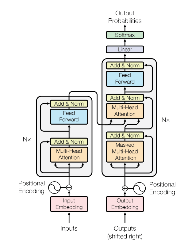
In the above diagram, there are two major parts: an Encoder stack (left) and the Decoder stack (right). The encoder turns input tokens into rich contextual embeddings, and the decoder stack generates the output tokens automatically. Each stack is built by repeating the same layer N times (e.g., 6, 12, 24…) to make the model deeper.

input tokens → input embedding + positional encoding → encoder layers (self-attention + FFN) → encoder outputs decoder receives shifted output embeddings + pos encoding → masked self-attention → encoder–decoder attention → FFN → linear → softmax → token probabilities.

Input embedding + positional encoding

In a Transformer, the input embedding is how words or tokens from your text are turned into numbers so the model can understand them. It’s like translating language into a secret code that the model speaks.

However, this code alone doesn’t tell the model where each word appears in the sentence. That’s where positional encoding comes in: it adds special numeric patterns to the embeddings to indicate the position of each token (first, second, third, etc.) in the sequence. By combining the two, the model knows both what each word means and where it is in the sentence, which is essential for understanding context and order.

Two common methods:

• Sinusoidal (fixed): PE(pos,2i)=sin(pos/10000^{2i/d}), PE(pos,2i+1)=cos(...).
• Learned: trainable position embeddings.

The sum of the token embedding + positional encoding is the input to the first encoder layer.

Encoder layer (one repeated block)

An encoder layer (one of the major parts) in a Transformer is a single building block that gets repeated multiple times (e.g., six times in the original Transformer). Each encoder layer has two main parts.

First is the multi-head self-attention mechanism, which allows every token in the input to look at every other token, figuring out how important each one is for understanding the current token’s meaning. This helps the model capture relationships like “who did what to whom” across the whole sequence.

The second part is a position-wise feed-forward network, which processes each token’s updated representation independently to transform and refine the learned features. Around both of these parts are residual connections (shortcuts that add the input back to the output) and layer normalization (which stabilizes learning), ensuring information flows smoothly and training remains stable. By stacking several identical encoder layers, the Transformer can build increasingly rich, context-aware representations of the input text.

Decoder layer (one repeated block)

A decoder layer in a Transformer consists of several identical blocks stacked on top of each other. It has three main parts. First, there is the Masked Multi-Head Self-Attention. In this part, each token in the decoder can only “see” earlier tokens and itself, using a look-ahead mask. This stops the model from looking at future words and ensures it generates text in a step-by-step manner.

Next is the Encoder–Decoder (Cross) Attention, where the decoder’s queries come from its previous layer, while the keys and values come from the encoder’s output. This setup lets the decoder focus on the most relevant parts of the input sentence as it generates each output token. Lastly, there is a Position-Wise Feed-Forward Network that refines the information for each token’s representation.

After each sublayer, the model applies Residual connections by adding the input back to the output and uses layer normalization (LayerNorm) to stabilize training. When the top decoder layer completes its work, its outputs pass through a linear projection and softmax, turning them into probabilities for each word in the vocabulary.

Attention: the core math (concise)

Linear Projections (per head)

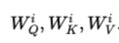
• Input sequence embeddings X (shape: seq_len × d_model) are projected into three different spaces:

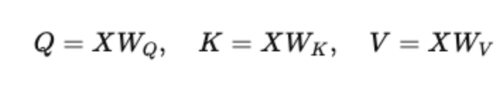
where WQ, WK, WV are learned weight matrices of shape (dmodel×dk).

• These projections let the model learn how to query, compare, and retrieve relevant information.

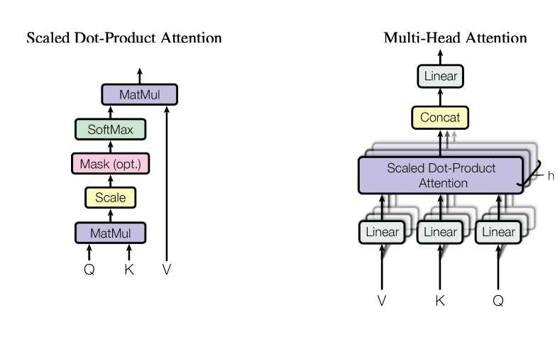
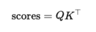
Scaled Dot-Product Attention

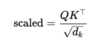
• Compute similarity scores between each query and all keys:

• Scale by dk​​ to avoid extremely large values that can make softmax unstable:

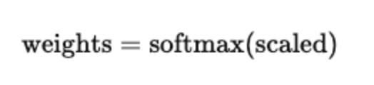
• Apply softmax across the key dimension to turn scores into attention weights:

• Multiply by V to get a weighted sum of value vectors.

Multi-Head Attention (MHA)

• Repeat the above process h times in parallel with different parameter sets,

• Each head focuses on different relationships or features in the sequence.
• Concatenate all heads’ outputs and project them back to dmodel space with WO​.

Masked Attention

Purpose: Prevent the model from looking at certain positions.

• Causal mask (future masking): In autoregressive tasks, block attention to tokens beyond the current position.
• Padding mask: Ignore padded positions in variable-length sequences.

How: Before softmax, add a large negative number (e.g., −∞) to the unwanted positions in the score matrix:

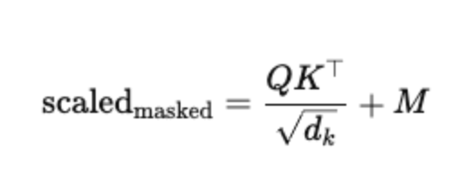
where M has 0s for allowed positions and −∞ for blocked ones.

• After softmax, these positions have near-zero probability.

Residuals, LayerNorm, and stability

In a Transformer, residual connections and layer normalization work together to keep training stable and efficient. A residual connection simply adds the sublayer’s input back to its output, ensuring that the original information is preserved and that gradients can flow backward more easily during training, which helps prevent vanishing or exploding gradients. Layer normalization then scales and shifts the combined output so that the values have a stable distribution, making learning smoother and faster. In the original Transformer, the order is Add → LayerNorm (post-norm), meaning normalization happens after the residual addition. Many newer models instead use pre-norm (LayerNorm → sublayer → Add), which tends to make very deep Transformers train more reliably by reducing the risk of unstable gradients. Together, these techniques keep the network from “forgetting” useful inputs while maintaining consistent activations across layers.

Output projection and loss

• The decoder’s final vectors are projected with a linear layer of shape (d_model, vocab_size) and a softmax to get token probabilities.
• Typical training uses teacher forcing: feed the true previous token to the decoder and compute cross-entropy loss between predicted distribution and the true next token.
• Weight tying: often the input embedding matrix and output linear weights are shared (transposed), which reduces parameters and helps convergence.

Masks in practice

In Transformers, masks are used to control what each token is allowed to “see” during attention. A padding mask is applied when sequences in a batch have different lengths; it blocks the model from paying attention to padding tokens that were added just to make all sequences the same size. A causal mask (also called a look-ahead mask) is used in the decoder to stop a token from looking at future tokens during training or generation, ensuring the model predicts text step-by-step without “cheating” by peeking ahead.

Key hyperparameters & typical sizes

• d_model (embedding + hidden dim): e.g., 512, 768, 1024, 2048…
• num_heads h: often 8 or 16; each head dimension = d_model / h.
• d_ff (FFN hidden dim): typically 4 × d_model (e.g., 2048 for d_model=512).
• Depth N: number of stacked layers (6, 12, 24, etc.).
• These choices affect compute, memory, and representational power.

Training Transformer models, whether for natural language processing, computer vision, or multimodal tasks, requires a lot of computational power. Transformers use multi-head attention, large matrix multiplications, and deep network layers that must process millions, or even billions, of parameters at the same time. On a CPU, these operations can take days or even weeks to finish, which makes model development and iteration extremely slow.

GPUs, or Graphics Processing Units, are built for high-throughput, parallel computation. This makes them perfect for speeding up Transformer training. Unlike CPUs, which are designed for sequential processing, GPUs have thousands of smaller cores that can perform many operations at once. This parallel setup greatly cuts down training time; tasks that might take weeks on a CPU can be completed in hours or days. For developers and researchers, this leads to faster experimentation and quicker iteration cycles. It also allows for training larger models without delays.

To make GPU power more accessible, GPU Droplets offer on-demand access to strong GPU instances, without the need to handle complex infrastructure. You can create an environment for AI/ML tasks in minutes and pay only for what you use.

DigitalOcean has modern, high-performance GPUs like the NVIDIA H100, designed for deep learning at scale. The H100 offers excellent throughput for Transformer architectures, enabling better training practices like mixed-precision computing, tensor cores, and high memory bandwidth. This is ideal for large-scale attention models and distributed training.

Set Up Local Environment: Create one if not done already, and add it to your DigitalOcean account.

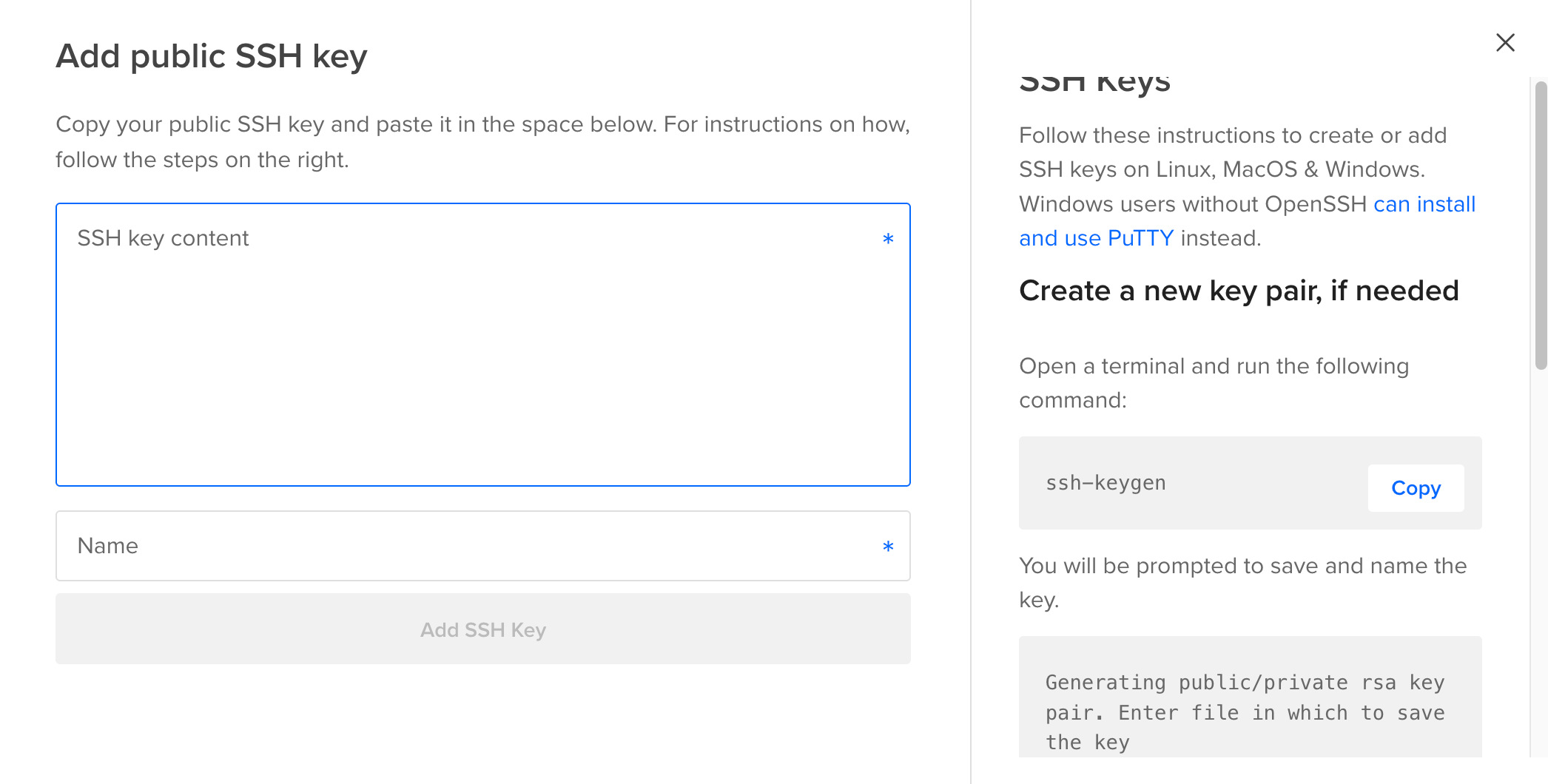
Refer to the “How to Add SSH Keys to New or Existing Droplets” documentation for detailed instructions on the process.

Install VS Code: Download VS Code for SSH connection and Jupyter integration.

Create GPU Droplet:

• Go to DigitalOcean and create a new Droplet.
• Datacenter: Choose a region closest to you.
• OS Template: Select AI/ML Ready.
• GPU Option: Choose Single H100 (enough for tutorial).
• SSH Key: Select or create one before starting.
• Name Your Droplet and create it.

SSH into the Droplet:

• Copy your Droplet’s IPv4 address from the dashboard.
• Run in terminal:

ssh root@<your IPv4 address>

Create New User & Install Dependencies:

useradd -m -g users <username>
su <username>
bash
cd ../home
apt install python3-pip python3.10-venv
pip3 install jupyterlab

Launch Jupyter:

jupyter lab

Connect via VS Code:

• Open VS Code
• Click “Connect to” → “Connect to Host” → “+ Add New SSH Host”.

ssh root@<your IPv4 address>

• Press Cmd + Shift + P → Search “Simple Browser” → Open it.
• Paste the Jupyter URL to view it locally.

You’ll now have JupyterLab running on your local browser with GPU acceleration from your DigitalOcean Droplet.

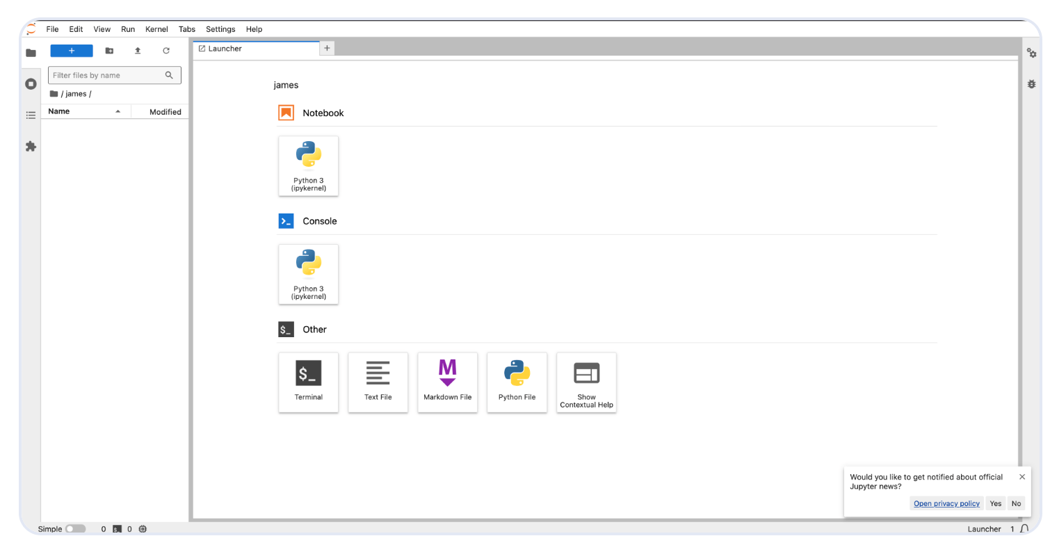
Check out the “Setting Up the GPU Droplet Environment for AI/ML Coding - Jupyter Labs” guide for a clearer overview of the steps.

Let us build a, light Transformer text classifier for the Kaggle “Disaster Tweets” dataset. Here we are using “Real or Not? NLP with Disaster Tweets” (easy to find on Kaggle). It has a text column and a binary target (0/1). You can swap in any similar CSV.

Before you run:

1. Download train.csv from the Kaggle dataset and place it in your working directory.
2. This script auto-splits train/val.
3. Run the script (or paste it into Jupyter).
4. Here we are using Python’s built-in re for tokenization.

Minimal Dependencies

pip install torch pandas scikit-learn numpy

Transformer Training Code

import re
import math
import random
import time
import os
import numpy as np
import pandas as pd
from collections import Counter
from sklearn.model_selection import train_test_split
from sklearn.metrics import accuracy_score, f1_score

import torch
import torch.nn as nn
from torch.utils.data import Dataset, DataLoader

# ====== Config ======
DATA_PATH = "./train.csv"  # Kaggle "Real or Not? NLP with Disaster Tweets"
MAX_LEN = 50
MIN_FREQ = 2
BATCH_SIZE = 64
EMBED_DIM = 128
FF_DIM = 256
N_HEADS = 4
N_LAYERS = 2
DROPOUT = 0.1
LR = 3e-4
EPOCHS = 5
SEED = 42
DEVICE = torch.device("cuda" if torch.cuda.is_available() else "cpu")

random.seed(SEED)
np.random.seed(SEED)
torch.manual_seed(SEED)

# ====== Load Dataset ======
df = pd.read_csv(DATA_PATH)[["text", "target"]].dropna()
train_df, val_df = train_test_split(df, test_size=0.15, stratify=df["target"], random_state=SEED)

# ====== Tokenizer & Vocab ======
def simple_tokenizer(text):
    text = text.lower()
    return re.findall(r"\b\w+\b", text)

counter = Counter()
for text in train_df["text"]:
    counter.update(simple_tokenizer(text))

# Special tokens
PAD_TOKEN = "<pad>"
UNK_TOKEN = "<unk>"
BOS_TOKEN = "<bos>"
EOS_TOKEN = "<eos>"

itos = [PAD_TOKEN, UNK_TOKEN, BOS_TOKEN, EOS_TOKEN] + [w for w, c in counter.items() if c >= MIN_FREQ]
stoi = {tok: i for i, tok in enumerate(itos)}

PAD_IDX = stoi[PAD_TOKEN]
BOS_IDX = stoi[BOS_TOKEN]
EOS_IDX = stoi[EOS_TOKEN]

def text_to_ids(text):
    tokens = [BOS_TOKEN] + simple_tokenizer(text)[:MAX_LEN-2] + [EOS_TOKEN]
    ids = [stoi.get(tok, stoi[UNK_TOKEN]) for tok in tokens]
    ids = ids + [PAD_IDX] * (MAX_LEN - len(ids)) if len(ids) < MAX_LEN else ids[:MAX_LEN]
    return ids

# ====== Dataset Class ======
class TextDataset(Dataset):
    def __init__(self, df):
        self.texts = df["text"].tolist()
        self.labels = df["target"].astype(int).tolist()
    def __len__(self):
        return len(self.texts)
    def __getitem__(self, idx):
        ids = torch.tensor(text_to_ids(self.texts[idx]), dtype=torch.long)
        label = torch.tensor(self.labels[idx], dtype=torch.long)
        return ids, label

train_ds = TextDataset(train_df)
val_ds = TextDataset(val_df)
train_loader = DataLoader(train_ds, batch_size=BATCH_SIZE, shuffle=True)
val_loader = DataLoader(val_ds, batch_size=BATCH_SIZE)

# ====== Positional Encoding ======
class PositionalEncoding(nn.Module):
    def __init__(self, d_model, max_len=5000):
        super().__init__()
        pe = torch.zeros(max_len, d_model)
        position = torch.arange(0, max_len, dtype=torch.float).unsqueeze(1)
        div_term = torch.exp(torch.arange(0, d_model, 2).float() * (-math.log(10000.0) / d_model))
        pe[:, 0::2] = torch.sin(position * div_term)
        pe[:, 1::2] = torch.cos(position * div_term)
        self.register_buffer("pe", pe.unsqueeze(0))
    def forward(self, x):
        return x + self.pe[:, :x.size(1), :]

# ====== Model ======
class TransformerClassifier(nn.Module):
    def __init__(self, vocab_size, embed_dim, num_heads, ff_dim, num_layers, num_classes, pad_idx, dropout=0.1):
        super().__init__()
        self.embedding = nn.Embedding(vocab_size, embed_dim, padding_idx=pad_idx)
        self.pos_encoding = PositionalEncoding(embed_dim)
        encoder_layer = nn.TransformerEncoderLayer(d_model=embed_dim, nhead=num_heads, dim_feedforward=ff_dim, dropout=dropout, batch_first=True)
        self.encoder = nn.TransformerEncoder(encoder_layer, num_layers=num_layers)
        self.fc = nn.Linear(embed_dim, num_classes)
    def forward(self, ids):
        mask = (ids == PAD_IDX)
        x = self.embedding(ids)
        x = self.pos_encoding(x)
        x = self.encoder(x, src_key_padding_mask=mask)
        x = x[:, 0, :]  # take BOS token
        return self.fc(x)

model = TransformerClassifier(len(itos), EMBED_DIM, N_HEADS, FF_DIM, N_LAYERS, 2, PAD_IDX, DROPOUT).to(DEVICE)
criterion = nn.CrossEntropyLoss()
optimizer = torch.optim.AdamW(model.parameters(), lr=LR)

# ====== Training Loop ======
for epoch in range(1, EPOCHS+1):
    model.train()
    train_loss = 0
    for ids, labels in train_loader:
        ids, labels = ids.to(DEVICE), labels.to(DEVICE)
        optimizer.zero_grad()
        output = model(ids)
        loss = criterion(output, labels)
        loss.backward()
        optimizer.step()
        train_loss += loss.item()
    
    # Validation
    model.eval()
    val_loss, preds_all, labels_all = 0, [], []
    with torch.no_grad():
        for ids, labels in val_loader:
            ids, labels = ids.to(DEVICE), labels.to(DEVICE)
            output = model(ids)
            loss = criterion(output, labels)
            val_loss += loss.item()
            preds_all.extend(torch.argmax(output, dim=1).cpu().numpy())
            labels_all.extend(labels.cpu().numpy())
    
    acc = accuracy_score(labels_all, preds_all)
    f1 = f1_score(labels_all, preds_all, average="macro")
    print(f"Epoch {epoch}: Train Loss={train_loss/len(train_loader):.4f}, Val Loss={val_loss/len(val_loader):.4f}, Acc={acc:.4f}, F1={f1:.4f}")

print("Training complete.")

# ====== Predict for a few random samples ======
model.eval()
sample_indices = random.sample(range(len(val_df)), 5)
for idx in sample_indices:
    text = val_df.iloc[idx]["text"]
    true_label = val_df.iloc[idx]["target"]
    ids = torch.tensor(text_to_ids(text), dtype=torch.long).unsqueeze(0).to(DEVICE)
    with torch.no_grad():
        pred = torch.argmax(model(ids), dim=1).item()
    print(f"Text: {text[:80]}...")  # print first 80 chars
    print(f"True: {true_label}, Pred: {pred}")
    print("-" * 50)

# ====== Save all validation predictions ======
all_preds = []
model.eval()
with torch.no_grad():
    for text in val_df["text"]:
        ids = torch.tensor(text_to_ids(text), dtype=torch.long).unsqueeze(0).to(DEVICE)
        pred = torch.argmax(model(ids), dim=1).item()
        all_preds.append(pred)

val_df_with_preds = val_df.copy()
val_df_with_preds["predicted"] = all_preds
val_df_with_preds.to_csv("validation_predictions.csv", index=False)
print("Saved validation predictions to validation_predictions.csv")

Let us discuss a few key points for the Transformer training code:

• Dataset Choice – If you are getting started it is recommended to use a lightweight, easy-to-download dataset (e.g., from Kaggle or Hugging Face Datasets) to avoid dependency conflicts.
• Tokenization – Apply a tokenizer (e.g., from transformers library) to convert text into numerical tokens suitable for the model.
• Model Selection – Feel free to select a small pre-trained Transformer model like distilbert/distilbert-base-uncased for faster training and fewer resource requirements.
• DataLoader Setup – Use DataLoader to efficiently batch and shuffle data for training and evaluation.
• Training Loop – Include forward pass, loss calculation (e.g., cross-entropy), backward pass, and optimizer step in each iteration.
• GPU Utilization – Move both the model and data to GPU (.to(device)) for faster training.
• Early Stopping – Implement early stopping to avoid overfitting when validation loss stops improving.
• Logging – Use tools like tqdm for progress bars and wandb or tensorboard for detailed experiment tracking.

1. What are Transformers, and why are they so popular?
Transformers are deep learning architectures that use self-attention to process input data in parallel, rather than sequentially like RNNs. This makes them highly efficient and scalable, allowing for breakthroughs in tasks like translation, summarization, and image classification. Their ability to capture long-range dependencies and handle large datasets has made them the go-to choice in modern AI research.

2. Why should I train Transformers on a GPU?
Transformers involve large matrix multiplications and attention computations, which are computationally heavy. GPUs are designed for parallel processing, which speeds up training dramatically. Without a GPU, training can take days or even weeks; with a GPU, it can be reduced to hours. DigitalOcean Gradient™ AI GPU Droplets allow you to instantly provision high-performance GPUs like the NVIDIA H100 for these workloads.

3. What is mixed precision training, and how does it help?
Mixed precision training uses a combination of 16-bit and 32-bit floating-point numbers during training. This reduces memory usage and speeds up computations without significantly affecting model accuracy, especially on GPUs with Tensor Cores optimized for FP16 operations.

4. How do I choose the right batch size for Transformer training?
Batch size affects training speed, convergence, and memory usage. A smaller batch size uses less memory but can make convergence noisier, while a larger batch size is more stable but memory-intensive. It’s often best to experiment with different sizes on your hardware.

5. Can I train a Transformer from scratch, or should I use pre-trained models?
Training from scratch is resource-intensive and requires large datasets. Most practitioners start with a pre-trained Transformer and fine-tune it on their specific dataset. Libraries like Hugging Face’s transformers make this process straightforward.

6. Why use DigitalOcean Gradient™ AI GPU Droplets for Transformer training?
They offer on-demand high-performance GPUs, quick setup, and integration with Jupyter Lab for interactive development. You can scale up when running large experiments and scale down when idle, optimizing costs without compromising performance.

In this guid, we explored the core concepts in a Transformer model, we understood the model architecture and few of the core concepts. We further understood the core steps of training the model from scratch which also included preprocessing the dataset to defining the model architecture and inference from the model.

While we focused on a relatively small and manageable dataset to demonstrate the concepts, the same principles can be applied to large-scale tasks as well. For production workloads, the ability to scale training efficiently becomes essential. This is where cloud GPU solutions can significantly accelerate your workflow.

DigitalOcean Gradient™ AI GPU Droplets provide a flexible, cost-effective way to train Transformer models without the need to maintain your own hardware. You’ll get the performance you need, only for as long as you need it, making it ideal for experimentation, fine-tuning, and production-level training.

Next Steps:

1. Play around with bigger datasets from places like Kaggle or Hugging Face Datasets.
2. Experiment with fine-tuning a pre-trained Transformer on a domain-specific task.
3. Implement more advanced optimizations such as learning rate warm-up, weight decay, or gradient clipping.
4. Apply more sophisticated optimizations like learning rate warm-up, weight decay, or gradient clipping.
5. Release your trained Transformer model on DigitalOcean App Platform or a GPU Droplet for real-time inference.

By combining strong model design with scalable GPU infrastructure, you can move from prototype to production faster and with less pain.

• Attention Is All You Need
• Vision Transformers (ViTs): Computer Vision with Transformer Models
• Transformers for Language Translation, Classification, and Segmentation Challenge
• A Comprehensive Guide to Byte Latent Transformer Architecture
• Transformer (deep learning architecture)
• Setting Up the GPU Droplet Environment for AI/ML Coding - Jupyter Labs