By Adrien Payong and Shaoni Mukherjee

Introduction
Proximal Policy Optimization (PPO) is one of the most widely used Reinforcement Learning algorithms over the past few years. It has been used as the go-to algorithm for numerous real-world deployments across various industries.
Developed by OpenAI, it has become popular in the research community and industry. PPO builds on the concept of policy gradient methods. However, it introduces new techniques to make the learning process more stable and efficient.
This article will guide you through the intricacies of PPO, from its mathematical foundations to practical implementation tips.
We will walk you through the inner workings of PPO, providing a deep understanding of the algorithm’s components, advantages, and limitations. Along the way, you’ll find hands-on code in PyTorch, and real-world deployment tips to help you get the most out of this powerful algorithm.
Key Takeaways
- PPO is the Gold Standard for Stability and Versatility Proximal Policy Optimization has been one of the most successful reinforcement learning algorithms since its introduction. This is owing to its stability and reliable training performance in both discrete and continuous action spaces. PPO’s clipped surrogate objective function prevents large updates that can destabilize the policy. This makes it a default algorithm of choice for robotics, games, and even fine-tuning large language models.
- Clipped Surrogate Objective is the Game Changer The key technical innovation of PPO is a clipped objective function that limits the amount of change to the policy at each training step. This clipping mechanism leads to a more conservative and stable learning update, reducing the likelihood of catastrophic performance collapse.
- Actor–Critic Architecture with Generalized Advantage Estimation Implementing PPO typically involves an actor–critic architecture, where the actor network suggests actions, and the critic evaluates them. Generalized Advantage Estimation (GAE) is used for computing advantages, which strikes a balance between bias and variance, providing more effective learning signals.
- Broad Real-World Adoption and Robust Performance Its relative simplicity, easy-to-tune nature, and strong empirical performance have led PPO to wide adoption in both research and industry. It is being used to train robotic arms, game-playing agents, autonomous vehicles, etc. It is also used for RLHF (Reinforcement Learning from Human Feedback) training of large language models such as ChatGPT.
- Hyperparameter Tuning and Common Pitfalls PPO is less sensitive to hyperparameter settings compared to earlier policy gradient methods. However, finding the right hyperparameters is still the key to good performance. The main hyperparameters to tune are the learning rate, clip range, entropy bonus, and batch size. Common pitfalls to watch out for include incorrect normalization, excessively large clip values, and unstable value function learning. Therefore, continuous monitoring and validation of the learning process is necessary.
Background: Policy Gradient Methods and Their Limitations
Reinforcement learning agents learn to make decisions by interacting with an environment, typically receiving feedback in the form of scalar reward signals. This is contrasted with supervised learning, which is based on labelled data. An RL agent typically explores, takes an action, and updates its policy many times in order to maximise total reward.
Policy gradient methods learn the policy directly, typically by gradient ascent on an objective function. The policy is a function that maps states to actions and is therefore suited to high‑dimensional continuous action spaces.
Classic policy gradient algorithms are known to be unstable. Single batch updates tend to move the policy far away from the data region. This leads to problems in generalizing from the data as well as recovering from bad updates.
Early stabilisation methods, such as Trust Region Policy Optimization (TRPO), enforced hard constraints on the KL‑divergence between policies at each step. TRPO, however, is complex and not compatible with neural network architectures that share parameters between the policy and value function. Proximal Policy Optimization was developed to solve these issues.
What is Proximal Policy Optimization?
PPO is a policy‑gradient algorithm that gently trains an agent to maximise expected returns. It performs this by updating the policy incrementally rather than taking large jumps. PPO achieves this by using a clipped surrogate objective, which prevents the new policy from deviating significantly from the old policy. The result is an objective function that allows for multiple gradient steps on collected trajectories without risk of policy collapse.
PPO is an on‑policy algorithm (it can only use data generated from the current policy, and can’t reuse old trajectories). The algorithm reliably converges if the KL‑divergence between the old and new policy is kept low.
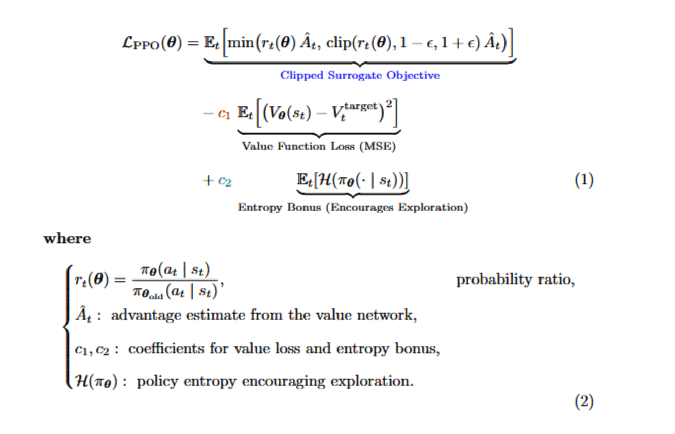
The Clipped Surrogate Objective
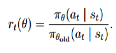
At the heart of PPO is the ratio of the new and old policy probabilities for a given action,
The vanilla policy gradient objective is multiplied by this ratio, weighted by the advantage At. PPO uses clipping (parametrized by a hyperparameter ϵ) to get the clipped surrogate objective:
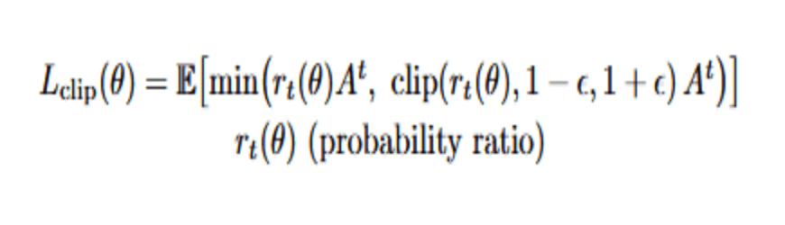
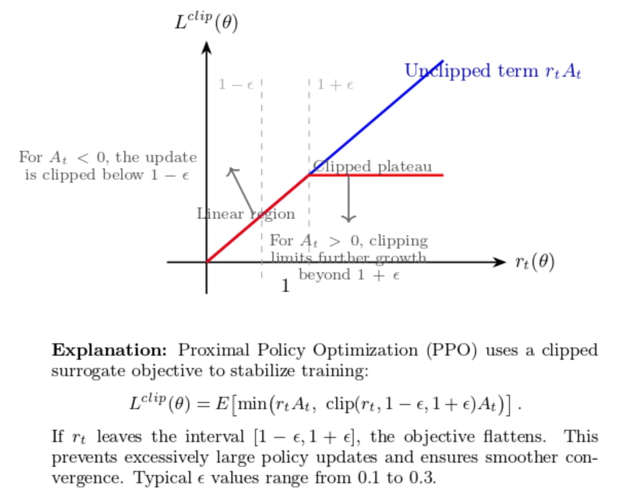
The objective takes the minimum of the unclipped and clipped terms. If rt falls outside of the interval [1−ϵ,1+ϵ], the clipped term truncates the objective. For positive advantages, pushing rt above 1+ϵ is not helpful as it no longer increases the objective. For negative advantages, pushing rt below 1−ϵ is similarly penalized. Since the optimizer maximizes the minimum of these two terms, the policy update is conservative and more stable. Typical values of ϵ are 0.1–0.3. The figure below shows how clipping truncates the objective outside of the allowed range.
Value function and advantage estimation
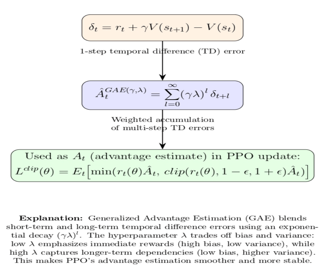
PPO is typically applied in an actor–critic style setup. A policy network (actor) that produces action probabilities, and a value network (critic) that estimates the expected return V(s). The advantage is calculated using Generalised Advantage Estimation (GAE), which takes multiple steps of temporal‑difference errors and combines them in a way that reduces variance.
The clipped objective also makes use of the value network in computing At. However, the value network is itself optimised via a mean‑squared error loss. PPO may also include an entropy bonus term to encourage exploration.
Step‑by‑Step Guide to Implementing PPO
Dividing PPO’s steps into separate components can also help understanding. A single iteration of the algorithm can be broken down into the following steps:
- Collect trajectories: Execute the current policy in the environment and store observations, actions, rewards, and log‑probabilities of the actions taken.
- Estimate returns and advantages: Often using Generalised Advantage Estimation to estimate the advantage of each action against a baseline.
- Compute the clipped surrogate loss: Compute the probability ratio and the clipped objective for each transition, then aggregate over the batch to form the policy loss.
- Update policy and value function: Take a gradient ascent step on the clipped objective and gradient descent step on the value loss (mean‑squared error between predicted and target values), optionally adding entropy regularization.
- Repeat: Collect new data from the environment using the updated policy and repeat until convergence.
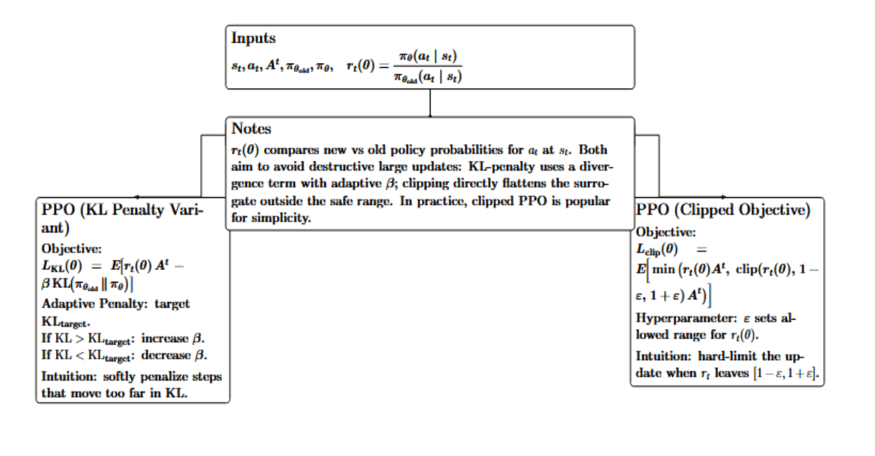
PPO has a KL penalty variant, which, instead of clipping, adds a KL penalty term to the objective, and adjusts the penalty coefficient adaptively so that the KL divergence approximately satisfies a target constraint. The clipped objective, however, is more popular because of its simplicity.
PPO Implementation in PyTorch
The code below may not be highly optimized. In practice, you might use established libraries (Stable Baselines3, Ray RLlib, CleanRL, etc.) for PPO. However, implementing from scratch is a great way to learn how PPO works under the hood.
We’ll implement PPO using PyTorch. We define an actor-critic network (shared backbone for policy and value), then train it on the CartPole-v1 environment from OpenAI Gym (now part of Gymnasium).
# --- compatibility shim for NumPy>=2.0 ---
import numpy as np
if not hasattr(np, "bool8"):
    np.bool8 = np.bool_

# --- imports ---
import gymnasium as gym   # use gymnasium; if you must keep gym
import torch
import torch.nn as nn
import torch.optim as optim

# Actor-Critic network definition
class ActorCritic(nn.Module):
    def __init__(self, state_dim, action_dim):
        super().__init__()
        self.fc1 = nn.Linear(state_dim, 64)
        self.fc2 = nn.Linear(64, 64)
        self.policy_logits = nn.Linear(64, action_dim)  # unnormalized action logits
        self.value = nn.Linear(64, 1)

    def forward(self, state):
        # state can be 1D (obs_dim,) or 2D (batch, obs_dim)
        x = torch.relu(self.fc1(state))
        x = torch.relu(self.fc2(x))
        return self.policy_logits(x), self.value(x)

# Initialize environment and model
env = gym.make("CartPole-v1")
obs_space = env.observation_space
act_space = env.action_space

obs_dim = obs_space.shape[0]
act_dim = act_space.n

model = ActorCritic(obs_dim, act_dim)
optimizer = optim.Adam(model.parameters(), lr=3e-4)

# PPO hyperparameters
epochs = 50               # number of training iterations
steps_per_epoch = 1000    # timesteps per epoch (per update batch)
gamma = 0.99              # discount factor
lam = 0.95                # GAE lambda
clip_epsilon = 0.2        # PPO clip parameter
K_epochs = 4              # update epochs per batch
ent_coef = 0.01
vf_coef = 0.5

for epoch in range(epochs):
    # Storage buffers for this epoch
    observations, actions = [], []
    rewards, dones = [], []
    values, log_probs = [], []

    # Reset env (Gymnasium returns (obs, info))
    obs, _ = env.reset()

    for t in range(steps_per_epoch):
        obs_tensor = torch.tensor(obs, dtype=torch.float32)

        with torch.no_grad():
            logits, value = model(obs_tensor)
            dist = torch.distributions.Categorical(logits=logits)
            action = dist.sample()
            log_prob = dist.log_prob(action)

        # Step env (Gymnasium returns 5-tuple)
        next_obs, reward, terminated, truncated, _ = env.step(action.item())
        done = terminated or truncated

        # Store transition
        observations.append(obs_tensor)
        actions.append(action)
        rewards.append(float(reward))
        dones.append(done)
        values.append(float(value.item()))
        log_probs.append(float(log_prob.item()))

        obs = next_obs
        if done:
            obs, _ = env.reset()

    # Bootstrap last value for GAE (from final obs of the epoch)
    with torch.no_grad():
        last_v = model(torch.tensor(obs, dtype=torch.float32))[1].item()

    # Compute GAE advantages and returns
    advantages = []
    gae = 0.0
    # Append bootstrap to values (so values[t+1] is valid)
    values_plus = values + [last_v]
    for t in reversed(range(len(rewards))):
        nonterminal = 0.0 if dones[t] else 1.0
        delta = rewards[t] + gamma * values_plus[t + 1] * nonterminal - values_plus[t]
        gae = delta + gamma * lam * nonterminal * gae
        advantages.insert(0, gae)

    returns = [adv + v for adv, v in zip(advantages, values)]

    # Convert buffers to tensors
    obs_tensor = torch.stack(observations)  # (N, obs_dim)
    act_tensor = torch.tensor([a.item() for a in actions], dtype=torch.long)
    adv_tensor = torch.tensor(advantages, dtype=torch.float32)
    ret_tensor = torch.tensor(returns, dtype=torch.float32)
    old_log_probs = torch.tensor(log_probs, dtype=torch.float32)

    # Normalize advantages
    adv_tensor = (adv_tensor - adv_tensor.mean()) / (adv_tensor.std() + 1e-8)

    # PPO policy and value update
    for _ in range(K_epochs):
        logits, value_pred = model(obs_tensor)
        dist = torch.distributions.Categorical(logits=logits)
        new_log_probs = dist.log_prob(act_tensor)
        entropy = dist.entropy().mean()

        # Probability ratio r_t(theta)
        ratio = torch.exp(new_log_probs - old_log_probs)

        # Clipped objective
        surr1 = ratio * adv_tensor
        surr2 = torch.clamp(ratio, 1 - clip_epsilon, 1 + clip_epsilon) * adv_tensor
        policy_loss = -torch.min(surr1, surr2).mean()

        # Value loss
        value_loss = nn.functional.mse_loss(value_pred.squeeze(-1), ret_tensor)

        # Total loss
        loss = policy_loss + vf_coef * value_loss - ent_coef * entropy

        optimizer.zero_grad()
        loss.backward()
        optimizer.step()
In the PyTorch code above, we follow the PPO algorithm structure:
- ActorCritic network: It returns policy logits and a value estimate. We implement this with two output layers at the top of shared hidden layers of size 64 (this is a very small network for CartPole).
- Data collection: We perform steps_per_epoch interactions. At each step, we sample an action from the policy (a Categorical distribution over discrete actions), take a step in the environment, and store the observations, actions, rewards, done flags, values, and log-probabilities. If the episode ends (done=True), we reset the environment and continue collecting until we’ve gathered the desired number of steps.
- Advantage and return calculation: After the batch is collected, we use GAE to compute advantages. We iterate backwards through the trajectory and accumulate the advantage estimate gae (the code implements GAE recursively using the formula delta + gamma*lam*…). We also compute the returns for each state (advantage + baseline value = total return estimate). Advantages are normalized (zero-mean, unit-std) to help training and numerical stability.
- PPO update: We take K_epochs passes of the batch through the network.
- Get the new log probabilities of the taken actions under the current policy (new_log_probs) and new value estimates value_pred.
- Compute the probability ratio = exp(new_log_prob - old_log_prob).
- Compute the clipped surrogate: surr1 (unchipped) and surr2 (clipped at 1±ε). We take the minimum of these for our policy loss. The negative sign is because we want to maximize the objective, but our optimizer does gradient descent (so we minimize the negative).
- Compute value loss as MSE between the predicted values and our computed returns.
- Add entropy bonus (weighted by 0.01 here) to encourage exploration by penalizing low entropy (subtracting because maximizing entropy is equivalent to subtracting entropy loss).
- Sum all these together to get the total loss, backpropagate, and update the network parameters with Adam.
The above implementation follows the spirit of PPO in that it uses the clipped objective (torch.min(surr1, surr2)) for the policy update, makes multiple passes of the same data, and keeps updates relatively small and safe.
PPO vs Other Algorithms (A2C, DQN, TRPO, etc.)
Here’s a rough, side-by-side comparison of PPO against some of the other widely used RL algorithms. Each row highlights the key concept behind the alternative approach, what PPO is generally better at, what the other method can be very good at (e.g., sample efficiency with replay in DQN (Deep Q-Network) or SAC (Soft Actor-Critic)/TD3), and when you’d typically choose PPO in practice.
| Comparison | Core Idea | PPO Advantages | When to Prefer PPO |
|---|---|---|---|
| PPO vs A2C/A3C | A2C/A3C: actor–critic without clipping; more hyperparameter-sensitive. | Clipped updates → higher stability; often better average scores; forgiving tuning. | General tasks where aggressive updates hurt; stable, smooth learning curves are needed. |
| PPO vs DQN | DQN: value-based, off-policy with replay; best for discrete actions. | Handles continuous actions; robust tuning; stochastic policies + entropy bonus. | Mixed/continuous action problems; prioritize stability and ease over sample efficiency. |
| PPO vs TRPO | TRPO: KL trust region via constrained, second-order optimization. | TRPO-like performance with simpler first-order clipping; lower compute. | Most practical settings need trust-region behavior without second-order solvers. |
| PPO vs SAC/TD3 | SAC/TD3: off-policy continuous control; replay; SAC maximizes entropy. | Very stable across tasks; simpler loop; fewer moving parts. | Debugging ease and robustness > peak sample efficiency; quick robotics baselines. |
| PPO in Large Action Spaces vs Value-Based | PPO scales to large discrete/continuous spaces without per-action Q updates. | Practical for massive/parameterized action spaces; multi-agent; long horizons. | Complex games/simulations with thousands of actions; multi-agent training. |
A study evaluating DQN, A2C, and PPO on Atari BreakOut found DQN got higher rewards quicker (smooth learning curve, high sample efficiency), while PPO and A2C took more time and were more exploratory/fluid in learning. However, DQN doesn’t generalize to environments with continuous actions or where there is a stochastic policy (e.g., robotic locomotion), and PPO excels in these due to its stability.
PPO provides a nice balance between simplicity, stability, and performance. If you need one algorithm that “just works” across many different environments, PPO is often the best choice. A2C may be simple but less stable. DQN may be more sample-efficient (in some settings) but only for discrete actions, and TRPO provides theory but little practical advantage over PPO. As such, PPO is now one of the most widely used RL algorithms.
Use Cases and Applications of PPO
PPO’s versatility has led to its adoption in many domains within reinforcement learning. Let’s consider the following table:
| Domain / Use Case | Typical Tasks & Action Space | Why PPO Works Well |
|---|---|---|
| Atari & Video Games | Arcade benchmarks (Pong, Breakout, etc.). 3D games (Unity, Doom). Discrete actions; frame-based inputs. | Stable learning over long training windows. Works well with parallel simulation. Often matches/exceeds older PG baselines. |
| Continuous Control & Robotics | Locomotion (HalfCheetah, Hopper, Walker, Humanoid). Manipulation, quadrotor flight. Continuous actions (Gaussian policy). | Robust updates via clipping. Fewer tuning headaches vs some off-policy methods. Strong baseline across many robot tasks. |
| Unity ML-Agents (Game AI / NPCs) | NPC behaviors, 3D navigation, multi-sensor agents. Single or multi-agent setups. | Default algorithm due to general stability. Handles visual observations & multiple agents. |
| Multi-Agent RL | Self-play, decentralized control. Very large state–action spaces | Clipping moderates unstable inter-agent updates. Proven in large-scale training (e.g., MOBA). |
| RLHF for Large Language Models | Fine-tuning LLMs with a learned reward model. Instruction following, preference alignment | Keeps updates close to the pretrained policy. Balances reward maximization & behavior preservation. Mature tooling (e.g., TRLX) |
| GRPO & Relative PPO Variants (LLMs) | Group/relative rewards; large-scale alignment. Math/Reasoning-focused fine-tuning. | Improved stability/efficiency for giant models. Demonstrated wins vs larger baselines. |
| Industry Applications | Robotics (manipulators, drones). Game AI with human-like behavior | Dependable baseline with minimal babysitting. Works across heterogeneous tasks. |
PPO is one of the algorithms that can be used for almost any RL task. Be it training a robot to walk, an agent to play a video game, or fine-tuning an AI assistant using human feedback. The basic concept of taking conservative updates when improving your agent’s behavior is incredibly useful in all of these settings. It’s the success across such a broad range of applications that has made PPO the gold standard in the RL community.
Hyperparameter tuning and common pitfalls
While PPO is relatively robust, there are still some pitfalls and hyperparameters to be mindful of. Here are some common issues and tips:
| Pitfall / Setting | Symptoms & Why It Matters | Recommended Defaults / Heuristics | Fix / Tip |
|---|---|---|---|
| Learning Rate Too High | Value loss diverges, policy collapses; entropy drops to ~0; reward flatlines or decreases. | Adam LR ≈ 3e-4 is a common stable default. |
Lower LR; monitor entropy/reward; consider LR schedules. |
| Improper Clip Range (ε) | ε too large (~0.5): almost no clipping → unstable updates. ε too small (~0.05): over-constrained → slow learning. | Start at ε = 0.2; consider 0.1–0.3 range. |
Tune ε; optionally decay ε over training for finer updates. |
| Batch Size & Epochs | Too small batch → noisy advantages; too large → slow cycles. Too many epochs → overfit on-policy batch; too few → under-train. | Timesteps/update: ~2048–4096 (Atari/MuJoCo). Update epochs: 3–10 (often 3–5). |
Scale batch via parallel envs; tune K_epochs to balance fit vs. on-policy freshness. |
| Advantage Normalization | Unnormalized large advantages dominate gradients → instability. | Normalize to mean 0, std 1, each update batch. | Always normalize Â; verify no leakage across batches. |
| Entropy Coefficient | Too high → agent remains random; too low/zero → premature, suboptimal determinism. | Start ~0.01; decay over time. |
Lower if high entropy with no learning; raise if early collapse. |
| Value / Policy Update Frequency | Critic lags → poor Â, weak policy updates; persistently high value loss. | Separate LR/epochs for actor vs critic (as in many libs). | Give the critic extra steps or a higher LR; monitor value loss closely. |
| Reward Scaling | Very large/small rewards → extreme advantages, gradient blow-up or vanishing. | Normalize or clip rewards; maintain reasonable magnitude. | Divide by a constant; use reward clipping/standardization. |
| Sparse Rewards | Few signals for on-policy learner → slow/no progress; exploration stalls. | High initial entropy; exploration aids. | Add intrinsic curiosity, reward shaping, curricula; increase entropy early. |
| Monitoring KL Divergence | Large KL despite clipping → policy changing too much; risk of instability. | Target KL ~0.01–0.02 per update (heuristic). |
Lower LR/ε; add early stop if KL exceeds target; adaptive LR. |
| Multithreading & Seeding | Parallel envs share seeds or desync updates → low diversity, brittle learning. | Unique seeds per env; synchronized rollout→update cycles. | Set per-env seeds; verify vectorized env logic; log seeds for reproducibility. |
PPO often fails due to misconfiguring a few knobs: learning rate, clip range, batch/epoch sizing, and exploration/advantage handling. Use a modest LR (≈3e-4), a clip value around 0.2, normalized advantages, large enough batches with 3–5 update epochs, and keep track of entropy and KL to ensure you’re “proximal.” PPO with reward scaling, a responsive critic, and clean seeding of parallel envs can often be trained without heavy tuning.
Pros and cons
To wrap up our exploration, let’s summarize the key advantages and disadvantages of PPO:
Advantages of PPO
- Simplicity: PPO is straightforward to implement and use, with no need for second‑order derivatives or constrained optimisation.
- Stability: The clipped surrogate objective caps the policy change, preventing excessive divergence and resulting in stable learning curves.
- Versatility: Can be applied to discrete and continuous action spaces and scales to high‑dimensional problems.
- Sample reuse: Enables multiple gradient updates on the same batch of data, making it more sample‑efficient than REINFORCE.
- Broad adoption: Widely adopted in robotics, games, RLHF, and research with numerous open‑source implementations (Stable Baselines3, Hugging Face TRL).
Disadvantages of PPO
- On‑policy: inability to use experience replay like off‑policy algorithms, resulting in lower sample efficiency than DQN or SAC.
- Value function dependency: Requires a separate critic network for the value function, which increases computation time and can lead to unstable value estimates, particularly in long sequence tasks.
- Sensitive to hyperparameters: Requires careful tuning of the clip parameter, learning rates, and entropy coefficient.
- Limited to single‑objective optimisation: with multi-objective RL, where objectives might be in conflict, it requires extensions (e.g., GCR‑PPO).
FAQ SECTION
-
How does PPO work in reinforcement learning? PPO is an algorithm that improves on traditional policy gradient methods by clipping the policy update to prevent destabilizing the agent. This results in more stable and reliable performance.
-
Why is PPO better than traditional policy gradient methods? PPO clips the policy update to avoid catastrophic policy changes, which can lead to more stable and reliable performance.
-
How does the clipping function improve stability? The clip range constrains how much the policy can change during each update, preventing wild parameter swings and reward collapse.
-
What are the key hyperparameters in PPO? The clip range (ϵ) coefficient, learning rate, value loss coefficient, entropy bonus, GAE lambda, batch size, and epochs per update.
-
Is PPO better than TRPO? PPO is easier to implement, has simpler code, and is faster than TRPO, with similar or better performance.
-
How is PPO used in robotics and gaming? PPO has been used to train robust and adaptive policies in continuous action spaces, such as controlling robotic arms and simulated agents. It can also be used to train competitive agents in games.
-
Can PPO be applied to large language models? Yes, PPO is the standard for RLHF (Reinforcement Learning from Human Feedback) training of large language models, used in models such as ChatGPT and Gemini.
-
What are common challenges when training with PPO? Common challenges include: Poor normalization, excessive clip range, inadequate batch sizes, and not learning the value function properly.
Conclusion
Proximal Policy Optimization is the gold standard algorithm for RL. It has become the go-to method for most applications due to its simplicity, stability, and generalizability. PPO’s clipped surrogate objective was a breakthrough that improved over older policy gradient algorithms. It addressed the instability and sensitivity issues associated with large policy updates without requiring the complex second-order optimization methods used in TRPO.
It is also well-suited for discrete, continuous, and high-dimensional action spaces. This makes it a default choice for various applications in robotics, games, autonomous systems, RLHF, and more. PPO may not be the most sample-efficient algorithm since it is an on-policy method. However, its primary strength lies in its stability and predictability, with limited need for hyperparameter tuning to achieve reliable learning dynamics and smooth convergence. This makes it an excellent choice when training stability is a priority and environments are sensitive to training disruptions. For further reading, you can look at the following resources:
Thanks for learning with the DigitalOcean Community. Check out our offerings for compute, storage, networking, and managed databases.
About the author(s)
I am a skilled AI consultant and technical writer with over four years of experience. I have a master’s degree in AI and have written innovative articles that provide developers and researchers with actionable insights. As a thought leader, I specialize in simplifying complex AI concepts through practical content, positioning myself as a trusted voice in the tech community.
With a strong background in data science and over six years of experience, I am passionate about creating in-depth content on technologies. Currently focused on AI, machine learning, and GPU computing, working on topics ranging from deep learning frameworks to optimizing GPU-based workloads.
Still looking for an answer?
This textbox defaults to using Markdown to format your answer.
You can type !ref in this text area to quickly search our full set of tutorials, documentation & marketplace offerings and insert the link!
 This work is licensed under a Creative Commons Attribution-NonCommercial- ShareAlike 4.0 International License.
Become a contributor for community
Get paid to write technical tutorials and select a tech-focused charity to receive a matching donation.

DigitalOcean Documentation
Full documentation for every DigitalOcean product.

Resources for startups and AI-native businesses
The Wave has everything you need to know about building a business, from raising funding to marketing your product.
The developer cloud
Scale up as you grow — whether you're running one virtual machine or ten thousand.

Start building today
From GPU-powered inference and Kubernetes to managed databases and storage, get everything you need to build, scale, and deploy intelligent applications.
