By Diogo Vieira and Anish Singh Walia

Introduction
Effectively sizing and configuring GPUs for vLLM inference starts with a clear understanding of the two fundamental phases of LLM processing, Prefill and Decode, and how each places different demands on your hardware.
This guide explains the anatomy of vLLM’s runtime behavior, clarifies core concepts like memory requirements, quantization, and tensor parallelism, and provides practical strategies for matching GPU selection to real-world workloads. By exploring how these factors interact, you’ll gain the knowledge needed to anticipate performance bottlenecks and make informed, cost-effective decisions when deploying large language models on GPU infrastructure.
Key Takeaways
-
Prefill vs. Decode phases determine hardware needs: The prefill phase (processing input prompts) is memory-bandwidth bound and affects Time-To-First-Token, while the decode phase (generating outputs) is compute-bound and determines token generation speed.
-
VRAM capacity sets absolute limits: Model weights and KV cache must fit within available GPU memory. A 70B model in FP16 requires 140GB for weights alone, making quantization essential for single-GPU deployments.
-
KV cache grows dynamically: Unlike static model weights, the KV cache expands based on context length and concurrency. A 70B model with 32k context and 10 concurrent users needs approximately 112GB for FP16 cache or 56GB for FP8 cache.
-
Quantization is the primary optimization lever: Reducing precision from FP16 to INT4 cuts memory usage by 75%, enabling large models to run on smaller GPUs. FP8 quantization offers the best balance of speed and quality on modern hardware.
-
Tensor Parallelism enables larger models: When models exceed single-GPU capacity, TP shards weights across multiple GPUs, pooling VRAM at the cost of communication overhead. Single-GPU execution is faster when feasible.
The Anatomy of vLLM Runtime Behavior: Prefill vs. Decode
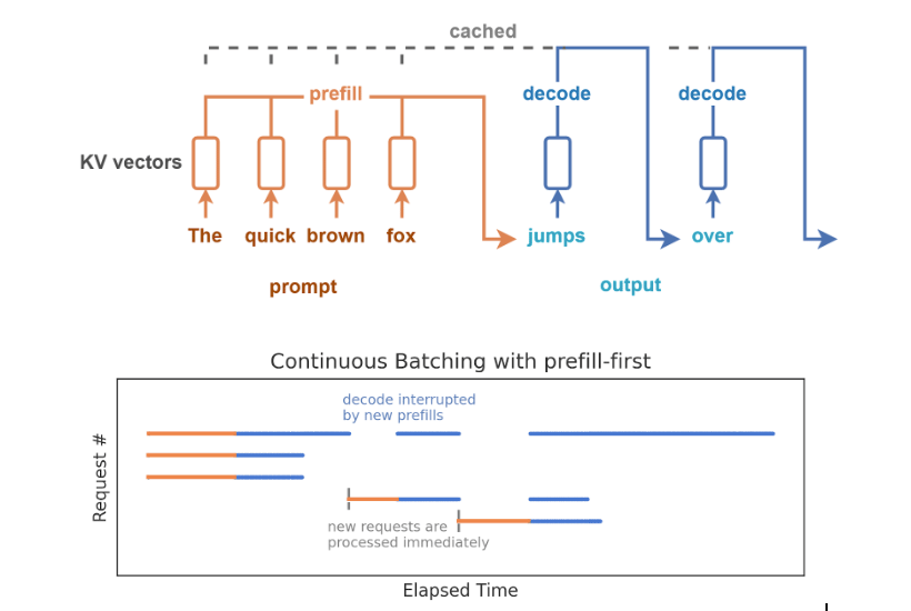
The Prefill Phase (“Reading”)
This is the very first step of any request. vLLM takes the entire input prompt (user query + system prompt + any RAG context) and processes it all at once in highly parallel fashion.
- What happens: The model “reads” the context and populates the Key-Value (KV) cache with the mathematical representation of that context.
- The Bottleneck: Because it processes thousands of tokens in parallel, this phase is almost always memory-bandwidth bound. The speed limit is how fast the GPU can move giant weight matrices from VRAM into the compute cores. For more on GPU performance characteristics, see our guide on GPU performance optimization.
- Real-World Impact: This determines Time-To-First-Token (TTFT). If you have a massive 100k token document to summarize, the prefill phase is what makes the user wait before the first word appears.
The Decode Phase (“Writing”)
Once the prefill is complete, vLLM enters an autoregressive loop to generate the output.
- What happens: The model generates one token, appends it to the sequence, and then runs the entire model again to generate the next token. This is inherently sequential for a single request.
- The Challenge: Loading enormous model weights from VRAM just to calculate a single token for one user is extremely inefficient; the GPU spends more time moving data than calculating.
- The Solution (Continuous Batching): To solve this, modern engines like vLLM do not process requests one by one. Instead, they use continuous batching. Requests enter and leave the batch dynamically. vLLM interleaves the prefill operations of new requests with the decode steps of ongoing requests in the same GPU cycle.
- The Bottleneck: When effectively batched, this phase becomes compute-bound (limited by raw TFLOPS), as the goal is to crunch as many parallel token calculations as possible to maximize total throughput.
Learn More: For a deeper analysis of static vs. continuous batching trade-offs, refer to this article: 🔗 Hugging Face: LLM Performance - Prefill vs. Decode
Linking Phases to Workloads & Hardware
Understanding which phase dominates your workload is essential for selecting the right hardware.
| Runtime Phase | Primary Action | Primary Hardware Constraint | Dominant Use Cases |
|---|---|---|---|
| Prefill | Processing long inputs in parallel. | Memory Bandwidth (TB/s) (Crucial for fast TTFT) | • RAG (Retrieval-Augmented Generation) • Long Document Summarization • Massive Few-Shot Prompting |
| Decode | Generating outputs sequentially. | Compute (TFLOPS) (Crucial for fast token generation) | • Interactive Chat & Customer Service • Real-time Code Generation • Multi-turn Agentic Workflows |
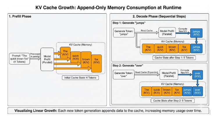
KV Cache at Runtime
During inference, vLLM relies heavily on a KV cache to avoid recomputing work it has already done.
- The Mechanics: In a transformer, each token is turned into key (K) and value (V) vectors inside the attention layers. Without a cache, the model would have to reprocess the entire history (tokens 0 … t) just to generate token t+1.
- The Solution: The KV cache solves this by storing the K and V vectors once and reusing them.
- Prefill: vLLM computes K/V for all prompt tokens and stores them immediately.
- Decode: For each new token, it retrieves the history from the cache and only computes the K/V for the new token.
- The Benefit: This turns attention from effectively quadratic work (re-reading the whole book to write every word) into linear work (just writing the next word).
The Trade-off: Dynamic Memory Growth: The price of this speed is memory. Every new token generated appends more entries to the cache. At runtime, KV cache usage grows dynamically based on:
- Prompt Length & Output Length: Longer conversations consume more VRAM.
- Concurrency: Each active request needs its own isolated cache.
- Model Size: Deeper models (more layers) and wider models (more heads) require larger caches per token.
Scaling Impact: This behavior is why two workloads using the same model can have vastly different hardware requirements. A 70B model might fit on a GPU, but if the KV cache grows too large during a long conversation, the server will run out of VRAM and crash. Understanding memory management is essential for production deployments, as covered in our fine-tuning LLMs guide.
Sizing Fundamentals: How Models, Precision, and Hardware Determine Fit
Once we understand how vLLM behaves at runtime, the next step is determining whether a model can run on a given GPU and what level of concurrency or context length it can support.
This section provides the mathematical formulas and decision trees needed to calculate static memory requirements, estimate KV cache growth, and systematically troubleshoot fit issues.
GPU Hardware Characteristics & Constraints
Before calculating model size, it is essential to understand the “container” we are trying to fit into. Different GPUs impose different hard limits on feasibility and performance.
Common Data Center GPU VRAM Capacities- These are the hard memory limits for the most common inference GPUs.
GPU Comparison for vLLM Inference and Training
| GPU Model | VRAM Capacity | Peak Dense TFLOPS (FP16 / FP8) | Primary Applications & Advantages |
|---|---|---|---|
| NVIDIA L40S | 48 GB | 362 / 733 | Cost-Effective Inference: Optimal for small-to-medium quantized models (7B–70B). |
| NVIDIA A100 | 40 GB / 80 GB | 312 / N/A | Previous Standard: 80GB version is excellent for tasks demanding high memory bandwidth. |
| NVIDIA H100 | 80 GB | 989 / 1,979 | Current High-End Standard: Features massive bandwidth, ideal for applications requiring long context lengths. |
| NVIDIA H200 | 141 GB | 989 / 1,979 | Significant Performance Boost: Allows for larger batch sizes or running 70B+ models with fewer required GPUs. |
| NVIDIA B300 | 288 GB | ~2,250 / 4,500 | Ultimate Density: Capable of fitting massive models (e.g., Llama 405B) with minimal GPU parallelism. |
| AMD MI300X | 192 GB | 1,307 / 2,614 | Massive Capacity: Perfectly suited for very large, unquantized models or processing huge batch sizes. |
| AMD MI325X | 256 GB | 1,307 / 2,614 | Capacity Optimized: Excellent choice for serving 70B+ models, especially those with very long context requirements. |
| AMD MI350X | 288 GB | 2,300 / 4,600 | High-Performance Flagship: Direct competitor to the B300, designed for massive-scale workloads. |
Even if a model fits in VRAM, the specific GPU architecture significantly impacts vLLM performance. Key metrics to consider are:
| Metric | Measured In | Impact on vLLM |
|---|---|---|
| VRAM Capacity | GB | Can it run? This sets the absolute maximum limit for the model size and context window. |
| Memory Bandwidth | TB/s | Prefill Speed. Crucial for RAG (Retrieval-Augmented Generation) and long-context summaries. High bandwidth ensures a fast Time-To-First-Token. |
| Compute (TFLOPS) | TFLOPS | Decode Speed. Essential for chat applications. High TFLOPS result in fast tokens/sec generation. |
| Interconnect | GB/s | Parallelism Cost. Any interconnect adds latency. Even with NVLink (DigitalOcean’s standard), Tensor Parallelism (TP) introduces synchronization overhead that reduces performance compared to single-GPU execution. |
Model Weight Footprint (Static Memory)
Every model must load its weights into GPU VRAM before vLLM can serve requests. The size of the weights depends entirely on the number of parameters and the precision chosen.
Formula for Static Weights
The estimated VRAM requirement (in GB) for a model can be calculated using the formula
**VRAM (GB) ≈ Parameters (Billions) × Bytes per Parameter
The table below illustrates the VRAM calculation for a Llama 3.1 70 Billion Parameter model at various quantization precisions
| Precision | Bytes per Parameter | Example: Llama 3.1 70B VRAM (GB) |
|---|---|---|
| FP16 / BF16 | 2 bytes | 70 x 2 = 140GB |
| FP8 / INT8 | 1 byte | 70 x 1 = 70GB |
| INT4 | 0.5 bytes | 70 x 0.5 = 35GB |
Precision choice is the single biggest lever for feasibility. Quantizing a 70B model from FP16 to INT4 reduces its static footprint by 75%, moving it from “impossible on a single node” to “fits on a single A100”. This makes quantization essential for cost-effective deployments on DigitalOcean GPU Droplets.
KV Cache Requirements (Dynamic Memory)
While weights determine if a model can start, the KV cache determines if it can scale. It is easy to underestimate the KV cache, leading to OOMs under load.
To accurately size a deployment, you need to estimate how much memory the cache will consume based on the expected context length and concurrency.
The “Field” Rule of Thumb (Quick Estimation)
For most customer conversations, the exact formula is too complex to calculate on the fly. Instead, use a “Per-Token” memory multiplier. This method gets you close enough for initial sizing decisions.
Simplified KV Cache Formula:
Total KV Cache (MB) = Total Tokens x Multiplier
(Where Total Tokens = Context Length x Concurrency)
Standard Multipliers:
| Model Size | Standard Multiplier (FP16 Cache) | Quantized Multiplier (FP8 Cache) |
|---|---|---|
| Small Models (7B - 14B) | 0.15 MB / token | 0.075 MB / token |
| Large Models (70B - 80B) | 0.35 MB / token | 0.175 MB / token |
Example Calculation:
A customer wants to run Llama 3 70B with a context of 32k and 10 concurrent users.
- Calculate Total Tokens: 32,000 x 10 = 320,000 tokens
- Apply Standard Multiplier (0.35): 320,000 x 0.35 MB = 112,000 MB 112 GB
- Check FP8 Option: If they enable FP8 cache, it drops to half: ~56 GB.
Verdict:
- FP16 Cache: 112 GB Cache + 140 GB Weights = 252 GB Total (Requires 4x H100s).
- FP8 Cache: 56 GB Cache + 140 GB Weights = 196 GB Total (Fits on 3x H100s, or tight on 2x H100s if weights are also quantized).
Exact Calculation & Tools
For detailed validation or corner cases, use the formal formula or an online calculator.
- Online Tool: LMCache KV Calculator
- Formal Formula:
Total KV Cache (GB) = (2 × n_layers × d_model × n_seq_len × n_batch × precision_bytes) / 1024^3
When Tensor Parallelism Is Required
Tensor Parallelism (TP) is a technique that shards (splits) a model’s individual weight matrices across multiple GPUs. Effectively, it allows vLLM to treat multiple GPUs as a single, massive device with pooled VRAM.
Why use it? TP is primarily a requirement for feasibility, not a performance optimizer. You typically enable it when:
- Weights don’t fit: The model is simply too big for one GPU (e.g., Llama 3 70B on a 24GB card).
- KV Cache limitations: The model fits, but leaves zero room for the KV cache, preventing you from running long contexts or high concurrency.
The “Tax” of Parallelism (Performance Impact) While TP unlocks massive memory, it introduces communication overhead. After every layer of computation, all GPUs must synchronize their partial results.
- If a model fits on one GPU: Running it on one GPU is almost always faster than running it on two. The single GPU has zero communication overhead.
- Interconnect Dependency: TP relies heavily on fast GPU-to-GPU bandwidth. If you use TP on cards without NVLink (e.g., over standard PCIe), inference speed can drop significantly due to synchronization latency. For deploying multi-GPU setups, consider using DigitalOcean Kubernetes to orchestrate your vLLM deployments.
Learn More: For a deeper look at how Tensor Parallelism shards models and impacts latency, refer to this conceptual guide: 🔗 Hugging Face: Tensor Parallelism Concepts
Putting the Numbers to the Test: Sizing Scenarios
Before moving to advanced configurations, let’s apply the math from the previous sections to real-world scenarios. This helps verify our understanding of “Fit” and introduces the practical constraints often missed in pure math.
The “Hidden” VRAM Tax
It is a common mistake to calculate Weights + Cache = Total VRAM and assume 100% utilization is possible. It is not.
- CUDA Context & Runtime: The GPU driver, PyTorch, and vLLM runtime reserve memory just to initialize (typically 2–4 GB).
- Activation Buffers: Temporary storage for intermediate calculations during the forward pass.
- Safe Sizing Rule: Always reserve ~4-5 GB of VRAM as “unusable” overhead. If your calculation leaves only 0.5 GB free, the server will likely crash.
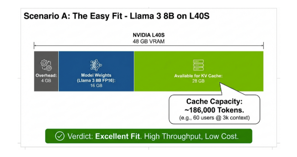
Scenario A: The Easy Fit (Standard Chat)
- Hardware: 1x NVIDIA L40S (48 GB)
- Model: Llama 3 8B (FP16)
- Math:
- Weights:
8B params x 2 bytes = 16 GB - Overhead:
-4 GB - Remaining for Cache:
48 - 16 - 4 = 28 GB
- Weights:
- Cache Capacity:
28,000 MB / 0.15 MB per token = 186,000 tokens.
- Verdict: Excellent Fit.
- This setup can handle massive loads (e.g., 60 concurrent users with 3k context each).
- Result: High throughput, low cost.
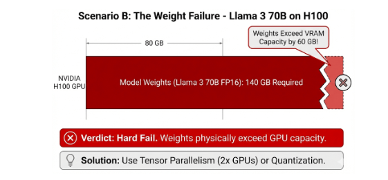
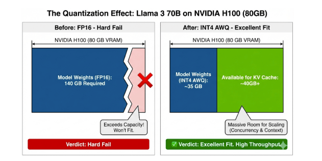
Scenario B: The “Weight Failure” (Large Model, Single GPU)
- Hardware: 1x NVIDIA H100 (80 GB)
- Model: Llama 3 70B (FP16)
- Math:
- Weights:
70B params x 2 bytes = 140 GB
- Weights:
- Verdict: Hard Fail.
- The weights (140 GB) physically exceed the GPU capacity (80 GB).
- Solution: You must use Tensor Parallelism (2x GPUs) or Quantization (Section 3).
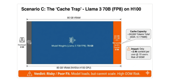
Scenario C: The “Cache Trap” (Fits, but cannot run)
- Hardware: 1x NVIDIA H100 (80 GB)
- Model: Llama 3 70B (FP8 Quantized)
- Math:
- Weights:
70B params x 1 byte = 70 GB - Overhead: -4 GB
- Remaining for Cache:
80 - 70 - 4 = 6 GB
- Weights:
- Cache Capacity:
6,000 / 0.175 MB per token (FP8) = 34,000 tokens total.
- Verdict: Risky / Poor Fit.
- The model loads, but you have almost no room to work.
- Impact: With 10 concurrent users, each gets only 3.4k context. If a user pastes a long document (4k tokens), the system will OOM.
- Lesson: Just because the weights fit, doesn’t mean the workload fits. This scenario usually requires a second GPU or a smaller model.
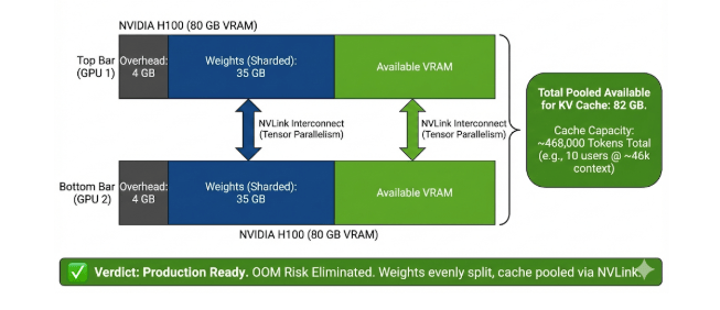
Scenario D: The Solution (Tensor Parallelism)
Let’s fix the “Cache Trap” from Scenario C by adding a second GPU. This demonstrates how Tensor Parallelism (TP) pools memory resources.
- Hardware: 2x NVIDIA H100 (80 GB each = 160 GB Total Available)
- Model: Llama 3 70B (FP8 Quantized)
- Math:
- Total VRAM: 160 GB
- Weights: -70 GB (Spread across both GPUs)
- Overhead: -8 GB (~4 GB per GPU)
- Remaining for Cache:
160 - 70 - 8 = 82 GB
- Cache Capacity:
82,000 / 0.175 MB per token (FP8) = 468,000 tokens total.
- Verdict: Production Ready.
- By adding a second GPU, we moved from a “risky” 6 GB of cache space to a massive 82 GB.
- Impact: With 10 concurrent users, each now gets ~46k context. The OOM risk is gone, and the deployment can handle RAG or long documents easily.
Quantization: The Art of “Squeezing” Models
As demonstrated in the previous sizing scenarios, VRAM is the primary bottleneck for LLM inference. Quantization is the technique of reducing the precision of the numbers used to represent data, effectively trading a tiny amount of accuracy for massive gains in memory efficiency and speed.
It is critical to distinguish between the two types of quantization used in vLLM, as they address different constraints.
Type 1: Model Weight Quantization (The “Static” Fix)
This involves compressing the massive, static weight matrices of the pre-trained model before it is loaded.
- Goal: Make a model fit onto a GPU where its full-precision weights would exceed VRAM capacity.
- vLLM Implementation: While vLLM can quantize weights dynamically at startup, it is generally more efficient to load a model that has already been quantized using high-performance kernels like AWQ (Activation-aware Weight Quantization) or GPTQ. These specialized formats offer better accuracy retention and faster decode speeds than generic on-the-fly conversion.
- Impact: Reduces static VRAM usage by 50% (FP8/INT8) to 75% (INT4/AWQ), significantly increasing the VRAM remaining for the KV cache.
Type 2: KV Cache Quantization (The “Dynamic” Fix)
This involves compressing the intermediate Key and Value states stored in memory during sequence generation.
- Goal: Make a model scale to support higher concurrent batches or longer context windows.
- vLLM Implementation: This is controlled via a runtime flag (
--kv-cache-dtype). - Recommendation: On modern hardware supporting FP8 tensor cores (e.g., NVIDIA H100, L40S, AMD MI300X), enabling FP8 KV Cache (
fp8) is highly recommended. It effectively doubles the available context capacity with negligible impact on model quality. - Impact: Halves the per-token memory requirement discussed in Section 2 (e.g., reducing the multiplier for a 70B model from ~0.35 MB/token to ~0.175 MB/token).
vLLM GPU Precision Formats
Not all quantization formats are created equal. The choice depends on the available hardware architecture and the desired balance between model size and accuracy.
| Precision / Format | Bytes per Param | Accuracy Impact | Best Hardware Support | Recommended Use Case |
|---|---|---|---|---|
| FP16 / BF16 (Base) | 2 | None (Reference) | All modern GPUs | The Gold Standard. Use whenever VRAM capacity permits. |
| FP8 (Floating Point 8) | 1 | Negligible | H100, H200, L40S, MI300X | Modern Default. The best balance of speed and quality on new hardware. Ideal for KV cache. |
| AWQ / GPTQ (INT4 variants) | ~0.5 | Low/Medium | A100, L40S, Consumer | The “Squeeze” Option. Essential for fitting huge models on older or smaller GPUs. Excellent decode speed. |
| Generic INT8 | 1 | Medium | Older GPUs (V100, T4) | Legacy. Generally superseded by FP8 on newer hardware or AWQ for extreme compression. |
Strategic Application & Trade-offs
Deciding when to apply quantization requires balancing practical constraints against workload sensitivity. While powerful, quantization involves fundamental trade-offs that must be considered during deployment planning.
Key Considerations: Accuracy & Hardware
Before determining the scenario, consider these two foundational constraints:
- Accuracy vs. Compression: Aggressive quantization (e.g., INT4) can degrade performance on sensitive tasks involving complex reasoning or code generation. FP8 is generally considered safe for most chat and RAG use cases.
- Hardware Compatibility: The chosen format must match the hardware’s capabilities. For example, FP8 quantization requires GPUs with FP8 tensor cores (NVIDIA Ada/Hopper or AMD CDNA3 architectures) to realize performance gains.
When Quantization Should Be Recommended
Based on the trade-offs above, quantization is appropriate in a wide range of real-world scenarios and is often the default choice in enterprise environments:
- Large models that don’t fit in FP16: INT4/INT8 is often the only way to serve 70B-class models on single 48GB or 80GB GPUs.
- High concurrency workloads: Reduced VRAM usage frees up significant space for the KV cache, allowing for more active sequences and longer prompts.
- RAG and enterprise chat: These workloads typically tolerate small accuracy deviations well without impacting the final user experience.
- Cost-optimization efforts: Quantization allows workloads to run on smaller, less expensive GPU SKUs while maintaining acceptable performance. This is particularly valuable when deploying on DigitalOcean GPU Droplets, where you can balance performance and cost based on your specific requirements.
When Quantization Should Be Avoided
Quantization is not universally suitable. Some workloads are highly sensitive to precision loss and should remain in FP16/BF16 whenever possible:
- Code generation and debugging: Lower precision can degrade structured reasoning, leading to subtle syntax errors or logical flaws.
- Math, finance, and scientific queries: Tasks requiring exact calculations benefit significantly from higher precision formats to avoid rounding errors.
- Evaluation, benchmarking, or regression testing: Small accuracy drift can invalidate comparisons between model versions or setups.
- Agentic workflows with multi-step reasoning: Compounded errors across multiple steps can reduce the system’s overall reliability and task completion rate.
Putting It All Together: From Requirements to a Deployment Plan
Up to this point, we have covered vLLM runtime behavior (Section 1), memory fundamentals (Section 2), and quantization strategies (Section 3).
This section connects these concepts into a repeatable decision framework. It moves from theory → practice, providing a structured workflow to evaluate feasibility, select hardware, and build a deployment plan.
Step 1: The Sizing Questionnaire
To accurately size a vLLM deployment, you must extract specific technical details from the workload description. Abstract goals like “fast inference” are insufficient. Use these five questions to gather the necessary data:
- “What is the maximum context length you need to support?”
- Why: Determines KV cache size (and thus, OOM risk).
- “What is your target concurrency (simultaneous users)?”
- Why: Multiplies the KV cache requirement.
- “What is the acceptable latency (TTFT and Tokens/Sec)?”
- Why: Determines if you need high bandwidth (H100) or just decent capacity (L40S).
- “Is model accuracy critical (Math/Code), or is ‘good enough’ acceptable (Chat)?”
- Why: Determines if you can use Quantization (INT4/FP8) to save money.
- “Do you have a hard budget constraint?”
- Why: Helps decide between optimizing for maximum speed (H100) vs. price-performance (L40S).
Step 2: Select Model Size and Precision
Once requirements are clear, identify the smallest model and highest precision that meets the quality bar.
- Precision is the Lever: Lower precisions (INT4/FP8) make large models feasible on cheaper hardware.
- The “Rule of 70B”: A 70B model in FP16 requires exotic hardware (multi-GPU). The same model in INT4 fits on commodity hardware (single GPU).
- Guidance:
- Chat/Assistant: Use INT4 or FP8.
- Code/Reasoning: Use FP16 or FP8 (Avoid INT4).
Step 3: Hardware Feasibility Check
Verify the fit using the math from Section 2.
- Static Fit (Weights): Does
Params * Precisionfit in VRAM?- If No: Quantize (Step 2) or add GPUs (Tensor Parallelism).
- Dynamic Fit (Cache): Is there room for
Context * Concurrency * Multiplier?- If No: Reduce concurrency, shorten context, or enable FP8 KV Cache.
- Workload Fit (Bandwidth):
- Long RAG/Summarization: Needs High Bandwidth (H100/A100).
- Standard Chat: Needs High Compute (L40S).
Step 4: Recommend the GPU Strategy
With feasibility confirmed, select the specific GPU SKU. Use this “Cheat Sheet” for common scenarios.
Common Configuration Outcomes
| Workload Scenario | Recommended Configuration | Rationale |
|---|---|---|
| Standard Chat (8B–14B) | NVIDIA L40S (48GB) | Best Value. Massive compute for decode; 48GB easily fits small models + huge cache. |
| Large Chat (70B, Cost-Sensitive) | L40S (INT4) or A100 (INT4) | The “Squeeze.” Quantization allows fitting 70B on a single card, avoiding the complexity of multi-GPU setups. |
| High-Performance Chat (70B) | NVIDIA H100 (FP8) AMD MI300X (FP16/FP8) | Modern Standard. H100 uses FP8 to fit and speed up inference. AMD Advantage: MI300X’s 192GB VRAM allows running 70B models with massive batch sizes on a single card. |
| Massive Context / RAG | NVIDIA H200 AMD MI300X / MI325X | Bandwidth & Capacity Kings. AMD: With 192GB (MI300X) or 256GB (MI325X), these are the best options for extreme context (128k+) without needing 4-8 GPUs. |
| Uncompromised Quality (70B FP16) | 2x H100 (Tensor Parallelism) 1x AMD MI300X | The “Single-Card” Hero. NVIDIA: Requires 2 cards to fit 140GB of weights. AMD: Fits the full 70B FP16 model on a single GPU, eliminating the latency penalty of Tensor Parallelism. |
| Ultra-Scale / Next-Gen (405B+) | NVIDIA B300 AMD MI350X | The Frontier. Designed for massive model density. MI350X (288GB) rivals NVIDIA’s Blackwell generation for fitting 400B+ MoE models efficiently. |
Step 5: Validate with Metrics
No paper sizing is perfect.
- Check TTFT: If high, your prefill is bottlenecked (bandwidth saturation).
- Check Inter-Token Latency: If high, your batch size might be too aggressive (compute saturation).
- Check KV Cache Usage: If consistently >90%, you are at risk of OOM and should enable Chunked Prefill or reduce concurrency.
Frequently Asked Questions
1. How much GPU memory do I need for LLM inference?
GPU memory requirements depend on model size, precision, context length, and concurrency. As a rule of thumb, FP16 models need approximately 2GB per billion parameters for weights alone. A 70B model requires 140GB for FP16 weights, but only 35GB with INT4 quantization. Additionally, you must account for KV cache memory, which grows with context length and concurrent users. For a 70B model with 32k context and 10 users, expect approximately 112GB for FP16 cache or 56GB for FP8 cache.
2. What is the difference between tensor parallelism and pipeline parallelism in vLLM?
Tensor parallelism (TP) shards model weight matrices across multiple GPUs within each layer, allowing multiple GPUs to work on the same computation simultaneously. This pools VRAM but requires synchronization after each layer, adding communication overhead. Pipeline parallelism (PP) distributes model layers across GPUs sequentially, with each GPU processing different layers. TP is typically used when a model is too large for a single GPU, while PP is more common in training scenarios. For inference, TP is the standard approach when models exceed single-GPU capacity.
3. When should I use quantization for vLLM deployments?
Quantization is recommended when models don’t fit in available VRAM, when you need to support higher concurrency or longer context windows, or when cost optimization is a priority. FP8 quantization is ideal for modern hardware (H100, L40S, MI300X) and offers minimal accuracy loss. INT4 quantization is necessary for fitting large models on smaller GPUs but should be avoided for code generation, math, and scientific tasks where precision matters. For chat and RAG workloads, quantization is often the default choice.
4. How do I calculate KV cache memory requirements?
Use the per-token multiplier method for quick estimation: multiply total tokens (context length × concurrency) by the model-specific multiplier. For small models (7B-14B), use 0.15 MB per token for FP16 cache or 0.075 MB for FP8 cache. For large models (70B-80B), use 0.35 MB per token for FP16 cache or 0.175 MB for FP8 cache. For exact calculations, use the formula: Total KV Cache (GB) = (2 × n_layers × d_model × n_seq_len × n_batch × precision_bytes) / 1024³, or use online tools like the LMCache KV Calculator.
5. Can I run vLLM on DigitalOcean GPU Droplets?
Yes, vLLM) can be deployed on DigitalOcean GPU Droplets. DigitalOcean offers GPU Droplets with NVIDIA GPUs that support vLLM’s requirements. When deploying, ensure your selected GPU has sufficient VRAM for your model size and workload. For cost-effective deployments, consider using quantized models (INT4 or FP8) to fit larger models on smaller GPU instances. DigitalOcean’s GPU Droplets provide NVLink connectivity, which is essential for efficient tensor parallelism when using multiple GPUs.
Practical Use-Cases of vLLM GPU Inference
Building on the foundational understanding of how factors like model size, precision, GPU architecture, KV cache, and batching influence performance, in the upcoming tutorials, we will apply these concepts to practical vLLM workloads.
For each use case, we will address three key questions to determine the optimal setup:
- Workload Definition: What are the defining characteristics? (e.g., prompt vs. output length, concurrency, latency sensitivity).
- Sizing Priorities: What factors are the bottleneck? (e.g., weights vs. KV cache, bandwidth vs. compute).
- Configuration Pattern: Which specific flags and hardware choices reliably perform well?
Use Case 1: Interactive Chat & Assistants
- Focus: Low Latency (Decode-Bound).
- Goal: Smooth streaming and fast “typing speed” for users.
- Key Constraint: Compute (TFLOPS) and Inter-Token Latency.
Use Case 2: High-Volume Batch Processing
- Focus: Max Throughput (Compute-Bound).
- Goal: Process millions of tokens per hour for offline jobs (e.g., summarization).
- Key Constraint: Total System Throughput (Tokens/Sec).
Use Case 3: RAG & Long-Context Reasoning
- Focus: Context Capacity (Memory-Bound).
- Goal: Fitting massive documents or history into memory without crashing.
- Key Constraint: VRAM Capacity and Memory Bandwidth (Prefill Speed).
Conclusion
Properly sizing and configuring GPUs for vLLM requires understanding the fundamental trade-offs between model size, precision, context length, and concurrency. The prefill and decode phases have different hardware requirements, with prefill demanding high memory bandwidth and decode requiring high compute throughput. Quantization serves as the primary lever for fitting large models on available hardware, while tensor parallelism enables scaling beyond single-GPU limits.
The key to successful deployment is matching your workload characteristics to the right hardware configuration. Interactive chat applications prioritize compute for fast token generation, while RAG and long-context workloads need massive VRAM capacity and high memory bandwidth. By following the sizing framework outlined in this guide, you can systematically evaluate feasibility, select appropriate hardware, and optimize your vLLM deployment for production workloads.
Next Steps
Ready to deploy vLLM on GPU infrastructure? Explore these resources to get started:
-
Deploy on DigitalOcean GPU Droplets: Get hands-on experience with vLLM by deploying on DigitalOcean’s GPU Droplets. Learn how to set up your environment and configure vLLM for optimal performance in our GPU Droplets documentation.
-
Related Tutorials: Deepen your understanding of LLM deployment and optimization:
- Run GPT-OSS vLLM on AMD GPU Droplet
- Learn about fine-tuning LLMs on a budget using DigitalOcean GPU Droplets
- Explore GPU performance optimization techniques for deep learning workloads
- Understand container orchestration for scaling LLM deployments
- Build a RAG application using GPU Droplets
-
Try DigitalOcean Products:
- GPU Droplets: High-performance GPU instances for AI and machine learning workloads
- DigitalOcean Kubernetes: Orchestrate and scale your vLLM deployments across multiple nodes
- DigitalOcean App Platform: Deploy and manage your LLM applications with ease
For more technical guides and best practices, visit the DigitalOcean Community Tutorials or explore our resources on AI and machine learning.
Thanks for learning with the DigitalOcean Community. Check out our offerings for compute, storage, networking, and managed databases.
About the author(s)
Senior Solutions Architect at DigitalOcean, helping builders design and scale cloud infrastructure with a focus on AI/ML and GPU-accelerated workloads. Passionate about continuous learning, performance optimization, and simplifying complex systems.
I help Businesses scale with AI x SEO x (authentic) Content that revives traffic and keeps leads flowing | 3,000,000+ Average monthly readers on Medium | Sr Technical Writer(Team Lead) @ DigitalOcean | Ex-Cloud Consultant @ AMEX | Ex-Site Reliability Engineer(DevOps)@Nutanix
Still looking for an answer?
This textbox defaults to using Markdown to format your answer.
You can type !ref in this text area to quickly search our full set of tutorials, documentation & marketplace offerings and insert the link!
 This work is licensed under a Creative Commons Attribution-NonCommercial- ShareAlike 4.0 International License.
Become a contributor for community
Get paid to write technical tutorials and select a tech-focused charity to receive a matching donation.

DigitalOcean Documentation
Full documentation for every DigitalOcean product.

Resources for startups and AI-native businesses
The Wave has everything you need to know about building a business, from raising funding to marketing your product.
The developer cloud
Scale up as you grow — whether you're running one virtual machine or ten thousand.

Start building today
From GPU-powered inference and Kubernetes to managed databases and storage, get everything you need to build, scale, and deploy intelligent applications.
