By Adrien Payong and Shaoni Mukherjee

Introduction
Deep learning frameworks have revolutionized artificial intelligence development by opening advanced techniques to a broader audience. Due to the availability of powerful open-source tools, developers and researchers can perform tasks such as image classification, speech recognition, and natural language processing.
MXNet has established a unique identity in the crowded field of deep learning frameworks. It excels through its hybrid programming model, cloud-native integrations, and GPU scalability. It’s also a mature production-ready engine that supports platforms like Amazon SageMaker and drives AI solutions across global enterprises.
This article will take you through the installation and basic usage of MXNet, multi-GPU scaling techniques, and deployment in production environments. It will provide benchmark comparisons between MXNet with frameworks like TensorFlow and PyTorch and tips to avoid typical errors.
Prerequisites
- Basic Python programming skills to understand and write MXNet Gluon code.
- Familiarity with deep learning principles, including neural networks, loss functions, and optimization processes.
- A Python environment with MXNet installed and the compatible MXNet package for your system’s CUDA version if using GPUs.
- A machine with CPU or GPU support is necessary, with additional setup of the CUDA toolkit and compatible drivers.
- A basic understanding of cloud service concepts( such as AWS or DigitalOcean) and containerization technologies like Docker for deploying machine learning models in production.
The Evolution of Apache MXNet
MXNet (“mix-net”) originated in 2015 within the Distributed Machine Learning Community at the University of Washington. The name itself highlights its goals: MXNet delivers a mix of flexibility for research and provides mobile and cloud platforms with efficient execution capabilities. The launch of MXNet as an official Apache Top-Level Project in 2017 recognized its strong governance structure, active community presence, and enterprise-level application potential.
Development Timeline:
- 2015: The Distributed (Deep) Machine Learning Community team at the University of Washington launched its first public release in 2015.
- 2016: The UW DMLC team collaborates with Amazon Web Services to enhance MXNet performance on AWS EC2 GPU systems.
- 2017: Graduation to Apache Top-Level Project.
- 2018–2020: Launching Gluon API for high-level imperative programming and significant developments in distributed training.
- 2021–Present: Integration with Apache TVM for deployment on edge devices, ONNX export capabilities, and core optimization efforts.
MXNet Architecture Overview
Understanding MXNet’s architecture is key to leveraging its full capabilities:
- NDArray: The n-dimensional array structure is the foundation for GPU operations and hybrid execution capabilities.
- Symbol and Computation Graph: Before execution, static computation graphs are optimized through operation fusion techniques and memory reuse strategies.
- Gluon (Imperative) API: The high-level interface enables smooth transitions from imperative to symbolic computation. The .hybridize() method allows deployment optimization without requiring code structure changes.
- KVStore and Parameter Server: A key-value store system that synchronizes parameters across devices and machines through multiple distributed modes.
- Executor and Backend Engine: The system compiles computation graphs while managing memory allocation and schedules asynchronous operations throughout available CPU and GPU resources.
- Gluon Blocks: Gluon Blocks offer modular components to build neural networks, allowing parameter tracking and custom forward pass definitions.
Below is a simplified diagram of MXNet’s data flow:
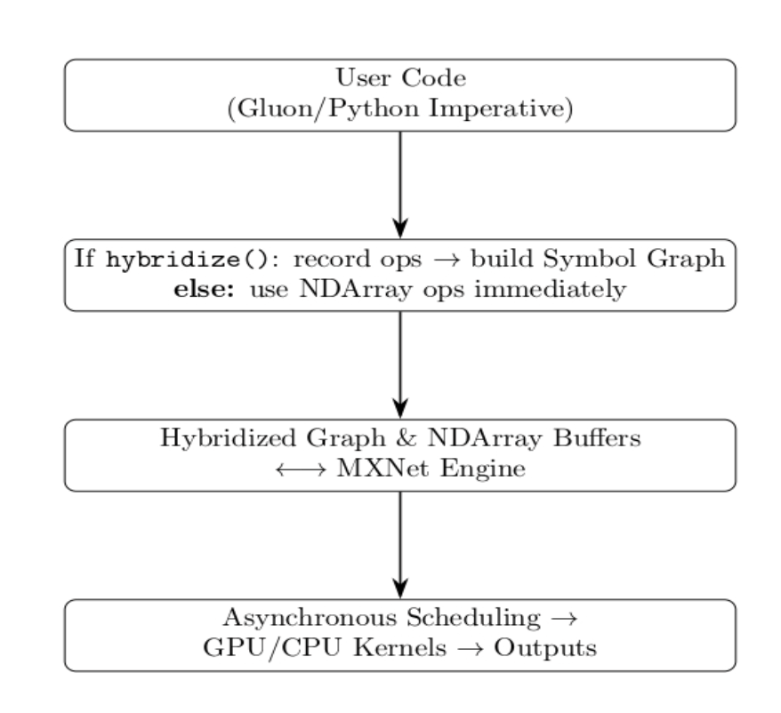
User Code (Gluon/Python Imperative): The Gluon model and training loop are implemented with Python.
Decision (hybridize vs. NDArray):
- Calling the net.hybridize() method causes MXNet to track all operations and build a static “Symbol Graph.”
- Otherwise, the model performs operations directly on NDArray objects (imperative mode) without graph optimization.
Hybridized Graph & NDArray Buffers ↔ MXNet Engine: MXNet’s core engine takes over the resulting graph (or live NDArrays) and data buffers to handle memory and computational resources.
Asynchronous Scheduling → GPU/CPU Kernels → Outputs: The engine performs asynchronous operation scheduling, which overlaps data transfers and computation before launching optimized kernels on the GPU or CPU that produce the final outputs.
Training a Deep Learning Model with MXNet Gluon
This section provides a straightforward example of how to train a deep learning model through MXNet Gluon. We will use the classic MNIST handwritten digits dataset for a basic neural network training.
Step 1: Installation and Setup If you haven’t already, you can install MXNet via pip. For example, to install the CPU-only version, use:
pip install mxnet
This installs MXNet with CPU acceleration. If you have an NVIDIA GPU and the CUDA toolkit installed, choose the MXNet package compatible with your CUDA version. For example, for CUDA 11.2:
pip install mxnet-cu112
The PyPI page displays individual packages based on each CUDA version. Use the command nvcc—-version to check your CUDA version and select the corresponding mxnet-cuXX package.
Note:
Ensure that your Python version is 3.6 or higher and that NumPy is up to date. On Linux systems, verify that libquadmath.so.0 is installed. For example, on Debian-based systems (including Ubuntu), you can usually install it using the following command:
sudo apt-get install libquadmath0
Note that some older MXNet pip packages may attempt to install outdated versions of NumPy, which can lead to installation failures. To avoid such issues, it is recommended to update both pip and numpy before installing MXNet.
Our example uses mxnet.gluon as the high-level neural network API, mxnet.nd for NDArray, and mxnet.autograd, which handles automatic differentiation.
import mxnet as mx
from mxnet import gluon, autograd, nd
Defining the device context for computations between the CPU and the GPU is a valuable approach. By default MXNet uses CPU. To Access GPU functionality, you must explicitly specify it:
ctx = mx.gpu() if mx.context.num_gpus() > 0 else mx.cpu()
The system will use the first available GPU; otherwise, it will fall back to the CPU. Multiple GPUs can be managed by using a list of multiple contexts, such as [mx.gpu(0), mx.gpu(1)]. However, in this section, we will stick to a single context.
Step 2: Loading the Data MXNet’s Gluon offers convenient data loading tools that make handling datasets straightforward. For example, the gluon.data.vision.datasets module can easily fetch some popular datasets. In this case, we’ll download the MNIST dataset and set up a data loader:
batch_size = 64

# Download the training dataset
train_dataset = gluon.data.vision.datasets.MNIST(train=True)
# Transform to normalize and convert images to tensors
transformer = gluon.data.vision.transforms.ToTensor()  # convert images to float32 tensor
train_data = gluon.data.DataLoader(train_dataset.transform_first(transformer),
                                   batch_size=batch_size, shuffle=True)
The code above provides an iterator, train_data, which supplies batches of 64 images with their labels, making it ready for training. In a real-world scenario, you’d typically create separate DataLoaders for validation and testing in a similar way.
Step 3: Defining the Model We will build a simple feed-forward network through Gluon’s nn (neural network) components. The gluon.nn.Sequential() container will be used to stack different layers.
net = gluon.nn.Sequential()
with net.name_scope():  # name_scope is optional but helps in naming layers
    net.add(gluon.nn.Dense(128, activation='relu'))   # Hidden layer with 128 units
    net.add(gluon.nn.Dense(64, activation='relu'))    # Hidden layer with 64 units
    net.add(gluon.nn.Dense(10))  # Output layer for 10 classes (0-9 digits)
The code above demonstrates a simple neural network featuring two hidden layers with ReLU activation functions, followed by an output layer with 10 units. While Gluon offers many pre-built layers—such as convolutional layers, LSTMs, and more—and a rich collection of pre-trained models in the Gluon model zoo, this basic network works perfectly for our current example.
Next, we’ll initialize weights with Xavier initializer and apply stochastic gradient descent (SGD) optimization with a learning rate of 0.1. The Gluon Trainer uses the model parameters with an optimization algorithm to perform updates. :
net.initialize(mx.init.Xavier(), ctx=ctx)  # initialize weights with Xavier initializer on the chosen context

loss_fn = gluon.loss.SoftmaxCrossEntropyLoss()       # Softmax cross-entropy for classification
trainer = gluon.Trainer(net.collect_params(), 'sgd', {'learning_rate': 0.1})
Step 4: Training Loop The training loop starts as we iterate through epochs and batches and perform forward and backward passes to update weights. Using Gluon’s autograd, this process becomes straightforward:
num_epochs = 3
for epoch in range(num_epochs):
    cumulative_loss = 0.0
    for data, label in train_data:
        data = data.as_in_context(ctx)     # move data to CPU or GPU
        label = label.as_in_context(ctx)   # move labels to the same context
        with autograd.record():            # start recording computation graph
            outputs = net(data)            # forward pass
            loss = loss_fn(outputs, label) # compute loss
        loss.backward()                    # backward pass (compute gradients)
        trainer.step(batch_size)           # update weights based on gradients
        cumulative_loss += loss.mean().asscalar()
    avg_loss = cumulative_loss / len(train_data)
    print(f"Epoch {epoch+1}, average loss: {avg_loss:.4f}")
A few things to note in this training code:
- During each iteration, we copy the data and labels to a GPU or CPU. MXNet requires users to move data to the correct device; if not, computations will default to running on the CPU.
- MXNet tracks operations for automatic differentiation through autograd.record(). Following the loss computation, we compute gradients for all parameters by calling loss.backward().
- The trainer.step(batch_size) optimization step updates all parameters. By passing batch_size, the MXNet Trainer performs accurate gradient averaging under the hood.
- We track training progress by accumulating the loss values. For each epoch, we print the average loss.
Running this training loop will output something like:
Epoch 1, average loss: 0.3469 Epoch 2, average loss: 0.1523 Epoch 3, average loss: 0.1092
indicating that the loss is decreasing. The model could achieve high accuracy scores on MNIST if trained across more epochs, with a decaying learning rate, or with an advanced network structure.
Multi-GPU Training on a Single Machine
MXNet simplifies multi-GPU training with minimal code changes. Below is a step-by-step example demonstrating how to leverage multiple GPUs effectively using MXNet’s Gluon API.
import mxnet as mx
from mxnet import gluon, autograd, nd

# 1. Detect available GPUs and create a list of contexts
gpu_count = mx.context.num_gpus()
ctx = [mx.gpu(i) for i in range(gpu_count)] if gpu_count else [mx.cpu()]

# 2. Define the neural network using HybridSequential
net = gluon.nn.HybridSequential()
with net.name_scope():
    net.add(
        gluon.nn.Dense(128, activation='relu'),
        gluon.nn.Dense(64, activation='relu'),
        gluon.nn.Dense(10)  # output layer for 10 classes
    )

# 3. Initialize parameters on all contexts and hybridize for performance
net.initialize(mx.init.Xavier(), ctx=ctx)
net.hybridize()

# 4. Define the loss function and trainer
loss_fn = gluon.loss.SoftmaxCrossEntropyLoss()
trainer = gluon.Trainer(net.collect_params(), 'adam', {'learning_rate': 0.001})

# 5. Training loop (assuming train_data is a DataLoader)
for data, label in train_data:
    # Split the batch evenly across GPUs/CPU contexts
    data_list = gluon.utils.split_and_load(data, ctx_list=ctx, even_split=True)
    label_list = gluon.utils.split_and_load(label, ctx_list=ctx, even_split=True)

    with autograd.record():
        losses = []
        for X, y in zip(data_list, label_list):
            X = X.reshape((-1, 784))        # Flatten input (e.g., for MNIST)
            y = y.as_in_context(ctx[0])     # Move labels to first context for consistency
            output = net(X)
            losses.append(loss_fn(output, y))
    for l in losses:
        l.backward()
    trainer.step(batch_size)
Explanation and Best Practices:
- Context Setup: The system automatically identifies available GPUs and generates a list of MXNet contexts (ctx). If no GPUs are detected, it automatically switches to CPU processing.
- Network Definition: HybridSequential defines the network structure to gain modularity and performance improvements. The net.hybridize() method compiles the network into a symbolic graph that optimizes speed and memory efficiency for training and inference processes.
- Data Splitting: split_and_load evenly distributes batches of data and labels to all available devices, allowing parallel processing.
- Label Context Management: The system moves labels to the first GPU context (ctx) to ensure consistency during loss computation.
- Backward Pass and Parameter Update: The trainer accumulates gradients from all GPUs by executing backward() on each loss and then performs a single parameter update once per batch.
- Scalability: This approach achieves near-linear scaling with the number of GPUs, which speeds training with minimal code changes.
Distributed Training Across Multiple Nodes
When the dataset or model size exceeds the capacity of a single machine, MXNet facilitates distributed training using two main approaches:
Built-in Parameter Server (KVStore)
MXNet’s built-in parameter server architecture allows you to scale training across multiple machines. Here’s how it works:
- Cluster Setup: Launch a scheduler and multiple server processes before starting worker processes on each individual node.
- Data Partitioning: Assign each worker a unique subset of the data to process. To ensure data is evenly distributed, you’ll need to specify parameters like `num_parts` and `part_index` for your data iterators, which handle data sharding properly.
- Parameter Synchronization: Workers send their computed gradients to parameter servers and retrieve updated weights during training. MXNet manages this process automatically, so you don’t need to worry about manual synchronization.
- Configuration: Enable distributed training within your training script through the following command-line: --kv-store dist_sync --num-servers <N> --kv-server-ip <IP>. The command line sets MXNet for distributed synchronous training with a parameter server (--kv-store dist_sync), the specified number of server processes (--num-servers <N>), and the server IP address (--kv-server-ip <IP>).
Horovod Integration
Horovod simplifies the parallelization of training tasks through workload scaling across distributed computing systems, multiple GPUs, or servers.
Installation:
pip install horovod[mxnet]
Initialization:
import horovod.mxnet as hvd
hvd.init()
ctx = mx.gpu(hvd.local_rank())
- Learning Rate Scaling: Remember to adjust your learning rate based on the total number of workers (hvd.size()).
- Trainer Setup: Use Horovod’s distributed store to wrap your Gluon Trainer and broadcast parameters to ensure every worker starts with the same model states.
- Launching Distributed Training: Launch the training script with the command `horovodrun -np 8 -H host1:4,host2:4 python train.py`. This command runs the script on 8 processes, distributing 4 processes per host, and running the train.py script on all.
Version Note: Some older MXNet versions may have issues integrating with Horovod, so it’s best to check compatibility before proceeding.
MXNet model deployment
Using trained MXNet models in production settings requires a series of important steps to ensure the model’s reliable deployment.
Persisting the Model
Once the model completes training, you should save the architecture and parameters to disk for future reproducibility and deployment.
net.export("cnn_mnist", epoch=0)
This command generates two essential artifacts:
- cnn_mnist-symbol.json: Contains the symbolic graph defining the network’s structure.
- cnn_mnist-0000.params: Stores the model’s parameters after training at the specified epoch.
Containerization with Docker
A typical Docker workflow for deploying MXNet models will look like this:
- Create the Dockerfile, which should use Python or MXNet runtime images, and include the required packages, inference scripts, and trained model files.
- Build the image locally: docker build -t my-mxnet-app .
- Test the container locally to ensure that inference operations perform correctly: docker run --rm my-mxnet-app
- After building the Docker image for your MXNet application, tag and push it to your container registry (e.g., DigitalOcean Container Registry).
- Deploy the image using your chosen platform — such as a Kubernetes cluster or DigitalOcean App Platform, for scalable inference serving.
This pattern establishes a deployment setup that provides robustness and portability for production-grade MXNet models.
Real-World MXNet Use Cases
The table below illustrates MXNet’s approach to solving various large-scale problems via effective model optimization and deployment methods.
| Use Case | Problem | Solution |
|---|---|---|
| Voice Assistants | Real-time speech-to-text (ASR) with low latency. | MXNet-optimized RNN/Transformer models on AWS EC2 instances, leveraging multi-GPU training and Multi Model Server for low-latency inference. |
| Autonomous Driving Research (Bosch, NVIDIA) | Process high-resolution sensor data (LiDAR, camera, radar) in real time. | Data parallelism across 128+ GPUs, hybrid graphs to optimize models, and ONNX export to run inference on NVIDIA Drive Orin platforms. |
| E-Commerce Recommendation Engines (Alibaba, Amazon) | Real-time personalization for hundreds of millions of users during shopping events. | Distributed training with parameter servers, large embedding tables, and hybridized candidate ranking models served via SageMaker. |
| Healthcare Imaging (NIH, Stanford Medicine) | Detect diabetic retinopathy or cancerous lesions from millions of high-resolution scans. | Fine-tune pretrained ResNet/Inception backbones using Gluon’s model zoo; export to ONNX and deploy on edge devices in clinics for immediate diagnosis. |
| Financial Fraud Detection (Ant Group, PayPal) | Analyze billions of transactions per day to flag anomalous patterns. | MXNet’s distributed data loading pipeline (HDFS + DataLoader), LSTM models for sequence analysis, and hybridized inference in a streaming environment (Apache Flink + ONNX). |
MXNet vs TensorFlow vs PyTorch: A Clear Comparison
The below presents a side-by-side comparison of the essential features for each framework:
| Aspect | MXNet | TensorFlow 2.x | PyTorch |
|---|---|---|---|
| API Style | Hybrid (Imperative + Graph) | Eager + Graph (tf.function) | Imperative (Eager) |
| Learning Curve | Moderate | Easy (Keras); advanced usage is more complex | Very low; Pythonic interface |
| Multi-GPU / Distributed | Native support + Horovod integration | MirroredStrategy + Horovod | Horovod, torch.distributed |
| Serving / Deployment | MXNet Model Server (MMS), SageMaker, ONNX | TensorFlow Serving, LiteRT, TF Hub | TorchServe, ONNX |
| Community | Growing; strong AWS support | Largest community and ecosystem | Research-centric community |
| Edge / Mobile | Apache TVM, ONNX | LiteRT, TensorFlow.js | TorchScript, ONNX |
| Performance | Leading for AWS; near-linear scaling | Excellent, especially on TPUs | Excellent for research workloads |
| Unique Strength | Hybridization and cloud-native design | TPU support; rich data-pipeline tools | Dynamic graphs and ease of debugging |
MXNet is a strong option for AWS SageMaker workflows, hybrid graph debugging, and GPU scaling with minimal code changes. TensorFlow is the better choice if you need TPU (Tensor Processing Unit) support. PyTorch commonly leads when it comes to research prototyping and aggressive model iteration.
Common Mistakes & How to Avoid Them
Even experienced developers sometimes face challenges when starting with a new framework. The table below outlines common mistakes in MXNet development and recommended best practices:
| Mistake | Impact | How to Avoid |
|---|---|---|
| Ignoring MXNet’s Gluon API | Reinventing the wheel; slower development. | Start all new projects with Gluon unless you have a legacy symbolic graph requirement. |
| Not Calling .hybridize() Before Inference | Slower inference; more CPU/GPU overhead. | After debugging, call net.hybridize() to compile the graph for production. |
| Mismatched Contexts Between Data & Model | CPU↔GPU transfers, crashes, and slowdowns. | Always send data (data.as_in_context(ctx)) and model parameters to the same device. |
| Neglecting DataLoader Optimizations | I/O bottlenecks slow down GPU utilization. | Use pin_memory=True, num_workers>0, and prefetch to overlap data loading. |
| Hardcoding Single-GPU Code | Scripts break when adding multiple GPUs or nodes. | Use split_and_load for multi-GPU and --kv-store flags for distributed training. |
| Forgetting to Tune Learning Rate for Multi-GPU | Divergence or suboptimal convergence. | Scale the learning rate by num_gpus (e.g., lr * num_gpus) per best practices. |
| Skipping Mixed Precision Training | Higher memory usage; slower speeds on modern GPUs. | Use mxnet.contrib.amp to enable FP16 mixed precision. |
| Not Using ONNX Export for Interoperability | Tied to MXNet only; harder to integrate with other services. | Export to ONNX with mxnet.contrib.onnx.export_model for wider runtime support. |
| Overlooking Parameter Server Configuration Flags | Inefficient or incorrect synchronization across nodes. | Pass appropriate --kv-store, --num-workers, and --num-servers flags. |
Taking proactive steps to resolve common pitfalls will help you achieve stable and efficient MXNet projects.
FAQ SECTION
What is MXNet used for? MXNet provides deep learning solutions for vision processing, natural language processing, speech recognition, recommendation systems, and reinforcement learning applicable to research environments and production settings.
Is MXNet better than TensorFlow? MXNet excels in AWS environments, hybrid execution, and scaling. TensorFlow leads in TPUs capabilities, ecosystem integration, and Big Data processing. The choice depends on your needs.
What programming languages does MXNet support? MXNet supports Python as its main language but allows developers to use Scala, Julia, R, C++, Perl, and JavaScript.
Does MXNet support GPU training? Absolutely. MXNet enables high-performance training on single GPUs and multiple GPUs while scaling easily to cluster environments.
How do I train a model? Begin by installing MXNet, setting the computation context, loading your data, and defining your model using Gluon. Then, initialize and hybridize the model, configure the loss function and optimizer, run the training loop with evaluation, and finally export the trained model.
Conclusion
MXNet is a scalable deep learning framework that provides flexibility and high-performance execution on CPUs, GPUs, and distributed systems. The combination of MXNet’s hybrid programming model, Gluon API, and integration with cloud services such as AWS SageMaker establishes it as a strong candidate for research and production use cases.
MXNet provides developers with multi-GPU training facilities and deployment support through MXNet Model Server and ONNX conversion to build efficient production-ready AI applications.
The following resources provide important insights and complementary knowledge for individuals looking to deepen their understanding of deep learning frameworks and model interoperability:
- What Every ML/AI Developer Should Know About ONNX
- What is Deep Learning?
- Popular Deep Learning Architectures: ResNet, InceptionV3, SqueezeNet
- PyTorch vs TensorFlow: A Detailed Comparison
Exploring these will further empower you to select and utilize the best tools for your AI projects.
References and Resources
- MXNet: A Flexible and Efficient Machine Learning Library
- Apache MXNet System Architecture
- Create a neural network
- Hybridize — MXNet Documentation
- Running inference on MXNet/Gluon from an ONNX model
- Container Registry Quickstart
- How to Use Your Private DigitalOcean Container Registry with Docker and Kubernetes
- How to Deploy from Container Images
Thanks for learning with the DigitalOcean Community. Check out our offerings for compute, storage, networking, and managed databases.
About the author(s)
I am a skilled AI consultant and technical writer with over four years of experience. I have a master’s degree in AI and have written innovative articles that provide developers and researchers with actionable insights. As a thought leader, I specialize in simplifying complex AI concepts through practical content, positioning myself as a trusted voice in the tech community.
With a strong background in data science and over six years of experience, I am passionate about creating in-depth content on technologies. Currently focused on AI, machine learning, and GPU computing, working on topics ranging from deep learning frameworks to optimizing GPU-based workloads.
Still looking for an answer?
This textbox defaults to using Markdown to format your answer.
You can type !ref in this text area to quickly search our full set of tutorials, documentation & marketplace offerings and insert the link!
 This work is licensed under a Creative Commons Attribution-NonCommercial- ShareAlike 4.0 International License.
Become a contributor for community
Get paid to write technical tutorials and select a tech-focused charity to receive a matching donation.

DigitalOcean Documentation
Full documentation for every DigitalOcean product.

Resources for startups and AI-native businesses
The Wave has everything you need to know about building a business, from raising funding to marketing your product.
The developer cloud
Scale up as you grow — whether you're running one virtual machine or ten thousand.

Start building today
From GPU-powered inference and Kubernetes to managed databases and storage, get everything you need to build, scale, and deploy intelligent applications.
