A Deeper Dive into Graph Neural Networks

• Graph Neural Networks (GNNs) work great for modeling relationships within interconnected data, making them ideal for tasks where structure and dependencies matter.
• GNNs generalize traditional deep learning to graph formats, allowing learning from nodes, edges, and their connectivity.
• Popular GNN architectures, such as Graph Convolutional Networks (GCNs), Graph Attention Networks (GATs), and GraphSAGE, offer different ways to aggregate and propagate information across nodes.
• Real-world applications of GNNs span social network analysis, molecular property prediction, recommendation systems, fraud detection, and knowledge graphs.
• Implementing GNNs is accessible with modern frameworks like PyTorch Geometric, which simplifies data handling, message passing, and model construction.
• A hands-on implementation demonstrates the GNN workflow, including loading graph data, defining a model, training, and evaluating results.
• GNNs continue to evolve rapidly, with advances improving scalability, efficiency, and performance in handling increasingly large and complex graphs.

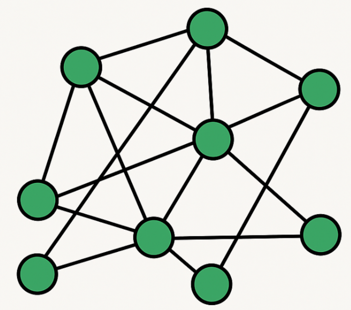
Graph Neural Networks, or GNNs for short, are a relatively new type of neural network that can work with data structured like graphs. Graphs are basically a bunch of objects, represented as nodes, and the relationships between those objects, represented as edges connecting the nodes, and GNNs can handle both directed graphs, where the edges have a direction, and undirected graphs, where the edges don’t have a specific direction. These graphs can vary significantly in size and shape as well. The architecture of a GNN consists of multiple layers, each of which takes information from the previous layer. We feed the GNN with a graph that is represented as a set of nodes and edges, along with their associated features. What we get out is a set of node embeddings for each node in the input graph. These embeddings represent the features the network learned for each node. Instead of just operating on vectors, matrices, or tensors like a normal neural network, GNNs can work with data structured as full-on graphs. That makes them really flexible for working with networked data, like social networks, molecular structures, or transportation systems. The math involved is complex, but the high-level idea is that they iterate through the graph, passing messages between nodes to learn useful representations.

Graph neural networks, or GNNs for short, are all about learning patterns between nodes in a network. The main idea is that each node passes messages to its neighboring nodes, sharing information about itself.

• In a GNN, each node exchanges information with the nodes it’s connected to, helping the model gradually understand the full graph structure.
• Every node creates a “message” using its own features and the features of its neighboring nodes.
• At the same time, neighboring nodes generate and send their own messages back.
• When a node receives these messages, it updates its internal state by aggregating all the incoming information.
• This repeated message-passing allows knowledge to flow through the graph, letting nodes learn about parts of the graph beyond their immediate neighbors.
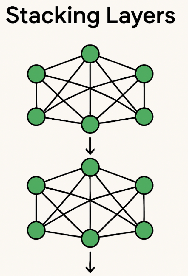
• By stacking multiple layers of this process, GNNs can learn more complex and deeper relationships.
• With each added layer, the model builds richer and more meaningful feature representations of the graph.

Cora dataset

The Cora dataset is a popular benchmark used by researchers working on graph representation learning. This dataset includes a bunch of scientific publications divided into seven categories like “Case Based,” “Genetic Algorithms,” “Neural Networks,” “Probabilistic Methods,” “Reinforcement Learning,” and "Rule Learning.” The Cora dataset has been around for some time and remains a go-to resource for many projects in this space. It provides a means to evaluate how effectively your model can analyze both the textual content of documents and the interconnected network of citations between them. Many notable graph neural network papers have utilized Cora to evaluate performance on these dual tasks. It’s built as a graph with the publications as nodes and citations between them as edges connecting the nodes. Each document is associated with a feature vector representing its content. The challenge here is to develop a model that can look at the citation graph, the content vectors, and the relationships between them in order to predict which of the seven classes any given publication belongs to.

We install the PyTorch Geometric library with the command:

pip install torch_geometric

We can then use the PyTorch Geometric library to load and preprocess the dataset.

from torch_geometric.datasets import Planetoid
import torch_geometric.transforms as T

dataset = Planetoid(root='data/Cora', name='Cora', transform=T.NormalizeFeatures())

The Planetoid class loads up the Cora dataset and normalizes the feature vectors. We can get the preprocessed data using the dataset, which gives us a Data object with these attributes:

• x: a matrix of node features of shape ‘(num_nodes, num_features )’
• edge_index: edge connectitivity matrix of shape ‘(2, num_edges)’
• y: a vector of node labels of shape ‘(num_nodes)’
• train_mask, val_mask, test_mask: boolean masks showing which nodes are for training, validating, and testing.

Model Architecture

When building a graph neural network, choosing the right model architecture is super important. We will walk through a basic implementation using PyTorch’s torch_geometric library. We will utilize a graph convolutional network, which serves as a solid starting point for various graph learning tasks.

import torch
import torch.nn.functional as F
from torch_geometric.nn import GCNConv

class GNN(torch.nn.Module):
    def __init__(self, in_channels, hidden_channels, out_channels):
        super(GNN, self).__init__()
        # Define the first graph convolutional layer
        self.conv1 = GCNConv(in_channels, hidden_channels)
        # Define the second graph convolutional layer
        self.conv2 = GCNConv(hidden_channels, out_channels)
        # Define the linear layer
        self.linear = torch.nn.Linear(out_channels, out_channels)

    def forward(self, x, edge_index):
        # Apply the first graph convolutional layer
        x = self.conv1(x, edge_index)
        # Apply the ReLU activation function
        x = F.relu(x)
        # Apply the second graph convolutional layer
        x = self.conv2(x, edge_index)
        # Apply the ReLU activation function
        x = F.relu(x)
        # Apply the linear layer
        x = self.linear(x)
        # Apply the log softmax activation function
        return F.log_softmax(x, dim=1)

• In the above code, we imported torch and torch.nn. functional to get access to some useful neural net modules and functions. Then, we defined a GNN class inheriting from torch and nn. Module.
• In the init method, we defined two convolutional layers using the GCNConv module from PyTorch Geometric. This allows for easy implementation of graph convolutions. We have added a simple linear layer.
• The forward pass first passes the input through the two conv layers, each time applying ReLU activation. Then it goes through the linear layer and finally the log softmax to squash the outputs.

In a few lines of code, we can build a nice little graph neural network!

Obviously, this is a simple example, but we can see how PyTorch and PyTorch Geometric let us quickly prototype and iterate on graph neural net architectures. The GCNConv layers make it very easy to incorporate graph structure into our models.

Training

For training, we’ll use cross-entropy loss and the Adam optimizer. We can split up the data into training, validation, and test sets using those mask attributes on the Data object.

# Set the device to CUDA if available, otherwise use CPU
device = torch.device('cuda' if torch.cuda.is_available() else 'cpu')
# Define the GNN model with the specified input, hidden, and output dimensions, and move it to the device
model = GNN(dataset.num_features, 16, dataset.num_classes).to(device)
# Define the Adam optimizer with the specified learning rate and weight decay
optimizer = torch.optim.Adam(model.parameters(), lr=0.01, weight_decay=5e-4)

# Define the training function
def train():
    # Set the model to training mode
    model.train()
    # Zero the gradients of the optimizer
    optimizer.zero_grad()
    # Perform a forward pass of the model on the training nodes
    out = model(dataset.x.to(device), dataset.edge_index.to(device))
    # Compute the negative log-likelihood loss on the training nodes
    loss = F.nll_loss(out[dataset.train_mask], dataset.y[dataset.train_mask])
    # Compute the gradients of the loss with respect to the model parameters
    loss.backward()
    # Update the model parameters using the optimizer
    optimizer.step()
    # Return the loss as a scalar value
    return loss.item()

# Define the testing function
@torch.no_grad()
def test():
    # Set the model to evaluation mode
    model.eval()
    # Perform a forward pass of the model on all nodes
    out = model(dataset.x.to(device), dataset.edge_index.to(device))
    # Compute the predicted labels by taking the argmax of the output scores
    pred = out.argmax(dim=1)
    # Compute the training, validation, and testing accuracies
    train_acc = pred[dataset.train_mask].eq(dataset.y[dataset.train_mask]).sum().item() / dataset.train_mask.sum().item()
    val_acc = pred[dataset.val_mask].eq(dataset.y[dataset.val_mask]).sum().item() / dataset.val_mask.sum().item()
    test_acc = pred[dataset.test_mask].eq(dataset.y[dataset.test_mask]).sum().item() / dataset.test_mask.sum().item()
    # Return the accuracies as a tuple
    return train_acc, val_acc, test_acc

# Train the model for 500 epochs
for epoch in range(1, 500):
    # Perform a single training iteration and get the loss
    loss = train()
    # Evaluate the model on the training, validation, and testing sets and get the accuracies
    train_acc, val_acc, test_acc = test()
    # Print the epoch number, loss, and accuracies
    print(f'Epoch: {epoch:03d}, Loss: {loss:.4f}, Train Acc: {train_acc:.4f}, Val Acc: {val_acc:.4f}, Test Acc: {test_acc:.4f}')

The train function does one round of training and returns the loss. The test function checks how the model performs on the training, validation, and test sets and returns the accuracy. We trained the model for 500 epochs and printed the training and testing accuracies at each epoch.

Compute the accuracy of the GNN model

The code below defines a function to calculate how accurate the model is on the entire dataset. The compute_accuracy() function switches the model to evaluation mode, performs a forward pass, and predicts labels for each node. It compares these predicted labels with the ground truth labels and calculates the number of correct predictions. Then it divides the number of correct predictions by the total number of nodes in the dataset to get the accuracy percentage.

@torch.no_grad()
def compute_accuracy():
    model.eval()
    out = model(dataset.x.to(device), dataset.edge_index.to(device))
    pred = out.argmax(dim=1)
    correct = pred.eq(dataset.y.to(device)).sum().item()
    total = dataset.y.shape[0]
    accuracy = correct / total
    return accuracy

accuracy = compute_accuracy()
print(f"Accuracy: {accuracy:.4f}")

In this case, the model’s accuracy on the Cora dataset was 0.8006. This means that about 80% of the time, the model was able to correctly predict the class label. That’s pretty good, but not perfect. Accuracy gives us a quick, high-level view of how well the model is performing overall. But you have to dig deeper to really understand where it’s succeeding and where it’s struggling.

To gain a deeper understanding of the model’s effectiveness, it is recommended to consider other evaluation metrics such as precision, recall, F1 score, and confusion matrix. These metrics provide insights into the model’s performance on different aspects, such as correctly identifying positive and negative cases and handling imbalanced datasets. So while 80% accuracy is solid, we’d want more context before declaring this model a smashing success. The accuracy metric alone doesn’t provide the full picture of what’s happening under the hood. But it’s a good starting point for gauging performance.

Evaluation

We can evaluate how the GNN’s performing using stuff like accuracy, precision, recall, and F1 score. But, we can also visualize the node embeddings the model learns using t-SNE. It takes the high-dimensional embeddings and projects them into 2D, allowing us to visualize them.

# Import the necessary libraries
from sklearn.manifold import TSNE
import matplotlib.pyplot as plt

# Set the model to evaluation mode
model.eval()

# Perform a forward pass of the model on the dataset
out = model(dataset.x.to(device), dataset.edge_index.to(device))

# Apply t-SNE to the output feature matrix to obtain a 2D embedding
emb = TSNE(n_components=2).fit_transform(out.cpu().detach().numpy())

# Create a figure with a specified size
plt.figure(figsize=(10,10))

# Create a scatter plot of the embeddings, color-coded by the true labels
plt.scatter(emb[:,0], emb[:,1], c=dataset.y, cmap='jet')

# Display the plot
plt.show()

Note: The reader can run the code above. It will display a scatter plot that can be interpreted. The code uses t-SNE to show the learned node embeddings in a 2D scatter plot, which is a smart way to visualize high-dimensional data. Let’s walk through what’s going on:

• Each point in the plot represents a node in the dataset. The x and y axes are the two dimensions that t-SNE squeezed the embeddings into. The color of each point represents the true label of the corresponding node in the dataset.
• Nodes that have similar embeddings should have similar labels, so they’ll cluster together on the plot. On the flip side, nodes with very different embeddings will probably have different labels, so they’ll be farther apart.
• Overall, the plot provides a clear representation of the relationships between nodes based on their learned embeddings. You can see groups forming that must share some underlying similarity. It’s a handy way to peek inside the model and understand how it’s organizing concepts.

Potential Challenges and Considerations

• With 2708 nodes and 5429 edges, the Cora dataset is considered to be on the smaller side. This might hinder the GNN’s efficiency, necessitating the adoption of more advanced methods like data augmentation and transfer learning.
• The Cora dataset consists of one type of node and one type of edge, making it a homogeneous network. This may limit the GNN’s applicability when applied to more complex networks, which involve diverse node and edge types.
• Selecting appropriate values for hyperparameters, such as the number of hidden layers, the number of hidden units, and the learning rate, can significantly impact the performance of the GNN and require careful tuning.

FAQ

• 1. What is a Graph Neural Network (GNN)?

A GNN is a neural network designed to work with graph-structured data. It learns node, edge, or graph-level representations by aggregating information from neighboring nodes.

• 2. How is a GNN different from a traditional neural network?

Traditional networks handle grid-like data (images, sequences), while GNNs can model irregular, interconnected structures such as social networks or molecular graphs.

• 3. What types of problems are GNNs used for?

They are commonly used for node classification, link prediction, graph classification, recommendations, fraud detection, and molecular property prediction.

• 4. What is message passing in GNNs?

Message passing is the core mechanism where nodes exchange information with their neighbors, update embeddings, and learn contextual relationships.

• 5. Do GNNs scale well to very large graphs?

Scaling can be challenging due to memory and neighborhood expansion. Techniques like sampling (GraphSAGE), mini-batching, and distributed training help.

• 6. What programming libraries are best for implementing GNNs?

Popular frameworks include PyTorch Geometric (PyG) and Deep Graph Library (DGL), both offering ready-made layers and utilities for building GNN models.

• 7. Are GNNs suitable for real-time applications?

Yes, depending on model complexity. Lightweight architectures and sampling-based approaches help achieve near real-time performance.

• 8. Can GNNs handle dynamic or evolving graphs?

Yes, dynamic GNN variants can process graphs that change over time, useful for traffic forecasting, temporal recommendations, and anomaly detection.

• 9. What data preprocessing is required for GNNs?

You typically need to prepare adjacency information, node/edge features, and ensure the graph is properly formatted for your chosen library.

• 10. Are GNNs interpretable?

Interpretability is improving with tools like attention mechanisms and GNNExplainer, which highlight influential nodes and edges.

In this article, we walked through the core concepts behind Graph Neural Networks (GNNs) and explored how they can be applied across different domains. GNNs are uniquely suited for working with graph-structured data, enabling models to reason about complex relationships found in social networks, molecular graphs, transportation systems, and more.

To demonstrate these ideas in practice, we used the popular Cora dataset—a benchmark for graph learning. In this dataset, each publication is represented as a node, and the citations between them form the edges. Our objective was to use both the textual features of each paper and the citation links to predict its category.

We prepared the dataset using the PyTorch Geometric library, normalizing the feature vectors and splitting the data into training, validation, and test sets. We then built a simple GNN using graph convolutional layers, followed by a linear classifier, and trained it using cross-entropy loss with the Adam optimizer. Finally, we evaluated the model’s performance by measuring its accuracy.

While there are many additional techniques and improvements one could explore, this project offers a solid introduction to how GNNs operate and how effective they can be for learning from complex relational data.

• Constructing Neural Networks From Scratch: Part 1
• What is Deep Learning? A Beginner’s Guide to Neural Networks
• Deep Learning Architectures Explained: ResNet, InceptionV3, SqueezeNet
• PyTorch 101: Learn Deep Learning with PyTorch