Building sharp regression models with K-Means Clustering + SVR

• Hybrid modeling boosts accuracy: Combining K-Means clustering with SVR often outperforms using Linear Regression or SVR alone, especially when the data is unevenly distributed.
• Ideal for non-uniform data: This approach works best when data naturally forms groups or clusters rather than following a single global trend.
• Silhouette Coefficient guides cluster selection: Using the Silhouette Score helps determine the optimal number of clusters, improving the overall performance of K-Means.
• Cluster-specific SVR improves predictions: Training separate SVR models for each cluster allows the algorithm to learn more targeted patterns within each data group.
• Scalability may add complexity: With more features, clustering and modeling become more complex, but the method can still offer significant improvements over basic algorithms.
• Two-step prediction pipeline: The final workflow involves predicting the cluster first and then using the corresponding SVR model to generate the final output.

Regression is a statistical method used to predict a dependent variable (Y) using certain independent variables (X1, X2,… Xn). In simpler terms, we predict a value based on factors that affect it. One of the best examples can be an online rate for a cab ride. When examining the factors that influence price prediction, we find that they include distance, weather, day, area, vehicle type, fuel price, and more. It is difficult to come up with an equation that provides the rate of the ride because of these many factors playing a huge role in it. Regression comes to the rescue by identifying how much each feature, as we may call them in Machine Learning terms, affects and comes up with a model that can predict the rate of a ride. Now that we have the idea behind regression, let’s look at Linear Regression.

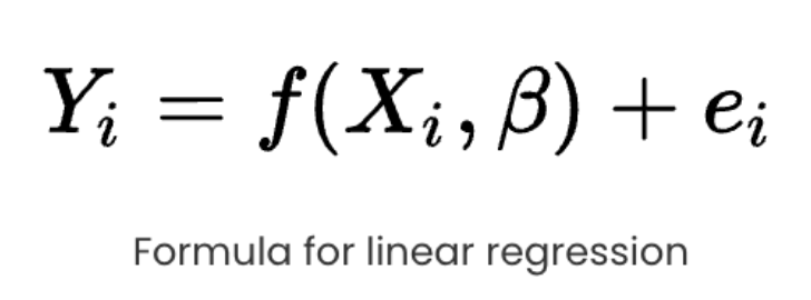
Linear regression is the go-to regression algorithm that aims at building a model that tries to find a linear relationship between independent variables (X) and the dependent variable (Y), which is to be predicted. From a visual point of view, we try to create a line such that points are at least a distance from it compared to all the other lines possible. Linear regression can handle only one independent variable, but the extension of linear regression, Multiple regression, follows the same idea with multiple independent variables contributing to predict the Y.

Even though linear regression is computationally simple and highly interpretable, it has its own share of disadvantages. It is only preferred when the data is linearly separable. Complex relations cannot be handled by this. A group of data points clustered in one region can highly influence the model, and a possible bias will occur. Now that we have understood what regression is and how the basic one works, let’s dive deep into some of the alternatives.

A decision tree is a tree where each node represents a feature, and each branch represents a decision. Outcome (numerical value for regression) is represented by each leaf. Decision trees are capable of capturing non-linear interactions between the features and the target variable. Decision trees are easy to understand and interpret. One of the major features is that they are visually intuitive. They are also capable of working with numerical and categorical features.

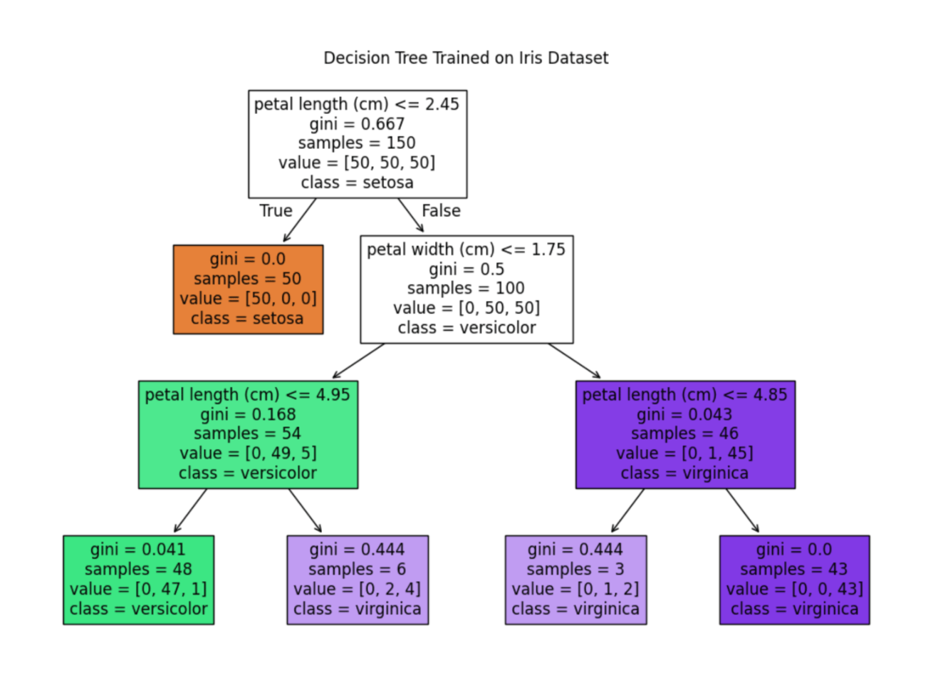
Some of the cons of using decision trees are that they tend to overfit. Even a small change in the data can cause instability because of the drastic change that might occur to the tree structure in the process.

Random Forest is a combination of multiple decision trees working towards the same objective. Each of the trees is trained with a random selection of the data with replacement, and each split is limited to a variable k features randomly selected with replacement on which to separate the data. This algorithm works better than a single decision tree in most cases. With multiple trees under the hood, the variations actually help in dealing with new data without any biases. Effectively, this allows a strong learner to be created from a collection of very weak learners. The final regression value is the mean of all the decision trees’ outcomes. With huge trees inside, it comes with certain downsides, such as slow execution while trying to achieve higher performance with all the trees. It also accounts for a huge memory requirement.

Now that we’ve covered the major regression algorithms, let’s shift our attention to the one at the core of this article: Support Vector Regression (SVR). SVR is a powerful technique known for its ability to control overall prediction error and remain robust in the presence of outliers, something simpler models like linear regression often struggle with. To understand how SVR works, it’s helpful to first look at the foundation it’s built on: Support Vector Machines (SVMs). Since SVR extends the principles of SVMs to regression tasks, getting familiar with the basic SVM intuition will make the SVR concepts much easier to grasp.

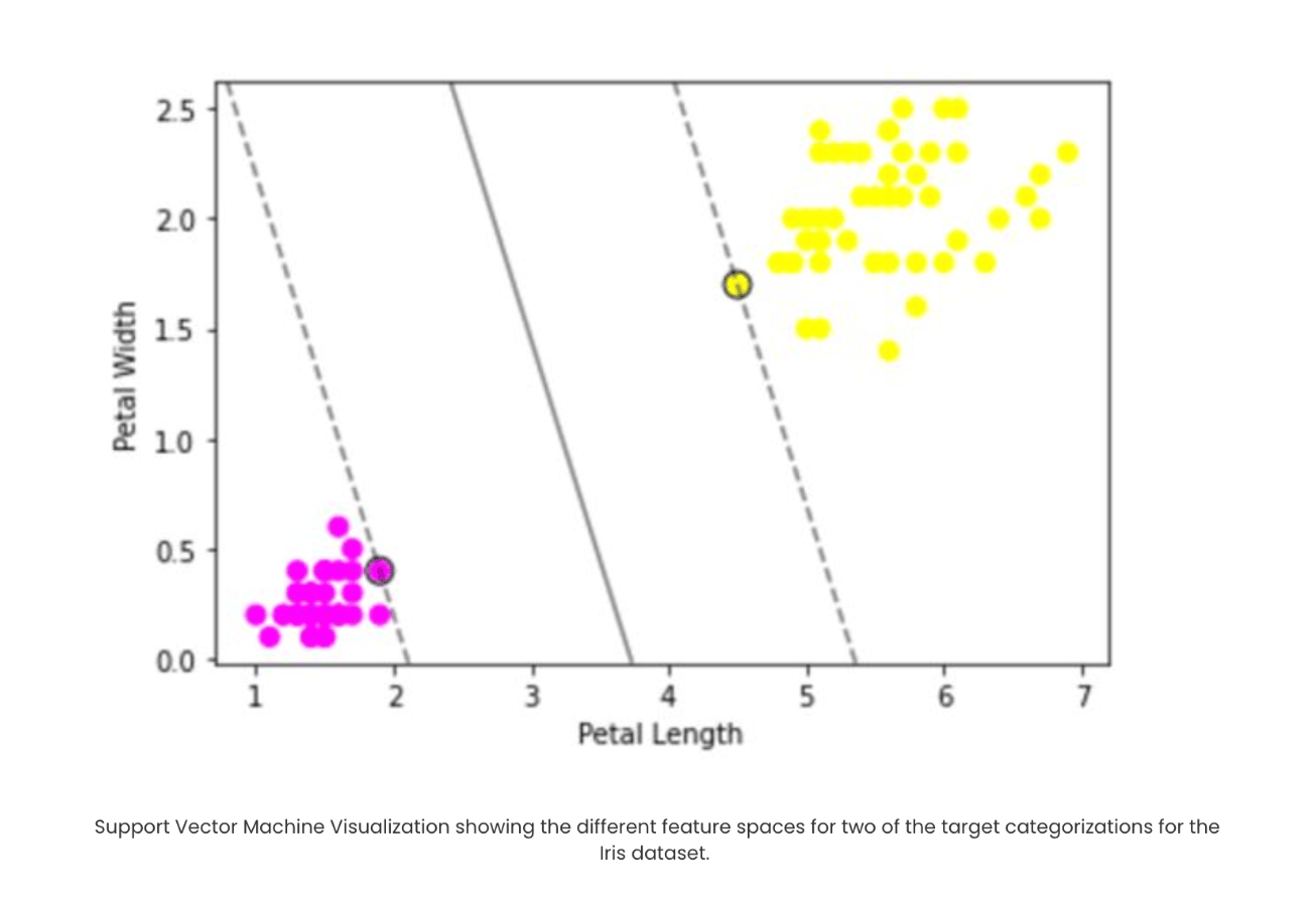
Support Vector Machine

Support Vector Machines (SVMs) aim to find a hyperplane in an N-dimensional feature space, where N is the number of input features, that can best separate the data points into different classes. What makes SVMs powerful is their ability to create a boundary that maximizes the distance between classes, instead of relying on a simple linear border like logistic regression often does. The goal is to position data points on either side of the hyperplane while treating those that fall too close to the boundary as outliers.

A key component that drives SVM’s performance is the kernel function. Kernels help transform the data into a higher-dimensional space where it becomes easier to separate the classes linearly. They also allow SVMs to scale effectively to high-dimensional datasets by computing the inner product of data points in this transformed space. Different kernels serve different types of data:

• The Gaussian (RBF) Kernel is ideal when we don’t know much about the underlying data structure.
• Linear Kernel works well when the data is already linearly separable.
• Polynomial Kernel captures relationships based on polynomial combinations of the input features.

These are just a few commonly used kernels, and there are many more that you can explore depending on the problem. Next, let’s look at a simple SVM implementation and visualize the hyperplane using the popular Iris dataset.

import seaborn as sns
from sklearn.svm import SVC 
import matplotlib.pyplot as plt
import numpy as np

# Creating dataframe to work on
iris = sns.load_dataset("iris")
y = iris.species
X = iris.drop('species',axis=1)
df=iris[(iris['species']!='versicolor')]
df=df.drop(['sepal_length','sepal_width'], axis=1)

# Converting categorical vlaues to numericals
df=df.replace('setosa', 0)
df=df.replace('virginica', 1)

# Defining features and targer
X=df.iloc[:,0:2]
y=df['species']

# Building SVM Model using sklearn
model = SVC(kernel='linear', C=1E10)
model.fit(X, y)

# plotting the hyperplane created and the data points' distribution
ax = plt.gca()
plt.scatter(X.iloc[:, 0], X.iloc[:, 1], c=y, s=50, cmap='spring')
ax.set(xlabel = "Petal Length",
       ylabel = "Petal Width")
xlim = ax.get_xlim()
ylim = ax.get_ylim()

xx = np.linspace(xlim[0], xlim[1], 30)
yy = np.linspace(ylim[0], ylim[1], 30)
YY, XX = np.meshgrid(yy, xx)
xy = np.vstack([XX.ravel(), YY.ravel()]).T
Z = model.decision_function(xy).reshape(XX.shape)

ax.contour(XX, YY, Z, colors='k', levels=[-1, 0, 1], alpha=0.5,
           linestyles=['--', '-', '--'])

ax.scatter(model.support_vectors_[:, 0], model.support_vectors_[:, 1], s=100,
           linewidth=1, facecolors='none', edgecolors='k')
plt.show()

Understanding SVR

Support Vector Regression uses the same principle as Support Vector Machine. SVR also builds a hyperplane in an N-dimensional vector space, where N is the number of features involved. Instead of keeping data points away from the hyperplane, here we aim to keep data points inside the hyperplane for regression. One of the tunable parameters is ε (epsilon), which is the width of the tube we create in the feature space. The next regularization parameter that we hypertune is C, which controls the “slack” (ξ ) that measures the distance to points outside the tube. Let’s see a simple implementation and visualization of SVR before we begin the combination of K-Means clustering and SVR. Here we are using the Real estate price dataset from Kaggle.

import pandas as pd
import numpy as np
from sklearn.svm import SVR # for building support vector regression model
import plotly.graph_objects as go # for data visualization
import plotly.express as px # for data visualization

# Read data into a dataframe
df = pd.read_csv('Real estate.csv', encoding='utf-8')
X=df['X2 house age'].values.reshape(-1,1)
y=df['Y house price of unit area'].values

# Building SVR Model
model = SVR(kernel='rbf', C=1000, epsilon=1) # set kernel and hyperparameters
svr = model.fit(X, y)

x_range = np.linspace(X.min(), X.max(), 100)
y_svr = model.predict(x_range.reshape(-1, 1))

plt = px.scatter(df, x=df['X2 house age'], y=df['Y house price of unit area'], 
                 opacity=0.8, color_discrete_sequence=['black'])

# Add SVR Hyperplane
plt.add_traces(go.Scatter(x=x_range, y=y_svr, name='Support Vector Regression', line=dict(color='blue')))
plt.add_traces(go.Scatter(x=x_range, y=y_svr+10, name='+epsilon', line=dict(color='blue', dash='dot')))
plt.add_traces(go.Scatter(x=x_range, y=y_svr-10, name='-epsilon', line=dict(color='blue', dash='dot')))

# Set chart background color
plt.update_layout(dict(plot_bgcolor = 'white'))

# Updating axes lines
plt.update_xaxes(showgrid=True, gridwidth=1, gridcolor='lightgrey', 
                 zeroline=True, zerolinewidth=1, zerolinecolor='lightgrey', 
                 showline=True, linewidth=1, linecolor='black')

plt.update_yaxes(showgrid=True, gridwidth=1, gridcolor='lightgrey', 
                 zeroline=True, zerolinewidth=1, zerolinecolor='lightgrey', 
                 showline=True, linewidth=1, linecolor='black')

# Update marker size
plt.update_traces(marker=dict(size=3))

plt.show()

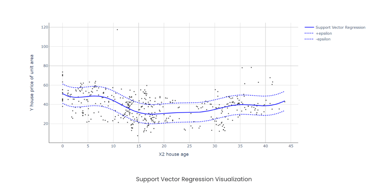
Here we can see that despite the non-linear distribution of data points, SVR neatly handled it with the hyperplane. This effect is even more apparent when we have more than one feature compared to other regression algorithms. Now that we have a good introduction to SVR, let’s explore the amazing combination of K-Means + SVR that can create wonders under the right regression circumstances.

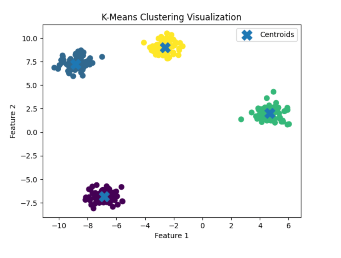
K-Means clustering is a popular unsupervised machine learning algorithm for clustering data. The algorithm works as follows to cluster data points:

• First, we define a number of clusters, let it be K here
• Randomly choose K data points as the centroids of the clusters
• Classify data based on Euclidean distance to either of the clusters
• Update the centroids in each cluster by taking the means of the data points
• Repeat the steps from step 3 for a set number of times (hyperparameter: max_iter)

Even though this seems pretty simple, there are a lot of ways to hypertune K-Means clustering. This includes correctly choosing the points to initialize centroids and a lot more. We will discuss one of them below, the Silhouette Coefficient, which provides a good indication of the number of clusters to choose from.

Implementing K-Means Clustering + SVR

We will be using the same Real estate price dataset from Kaggle for this implementation. Here, our independent variables are ‘X3 distance to the nearest MRT station’ and ‘X2 house age’. ‘Y house price of unit area’ is our target variable, which we will predict on. Let us first visualize the data points to define the need for clustering.

import pandas as pd # for data manipulation
import numpy as np # for data manipulation
import matplotlib.pyplot as plt

# Read data into a dataframe
df = pd.read_csv('Real estate.csv', encoding='utf-8')

# Defining Dependent and Independant variable
X = np.array(df[['X3 distance to the nearest MRT station','X2 house age']])
Y = df['Y house price of unit area'].values

# Plotting the Clusters using matplotlib
plt.rcParams['figure.figsize'] = [14, 7]
plt.rc('font', size=14)

plt.scatter(df['X3 distance to the nearest MRT station'],df['X2 house age'],label="cluster "+ str(i+1))
plt.xlabel("X3 distance to the nearest MRT station")
plt.ylabel("X2 house age")
plt.legend()
plt.show()

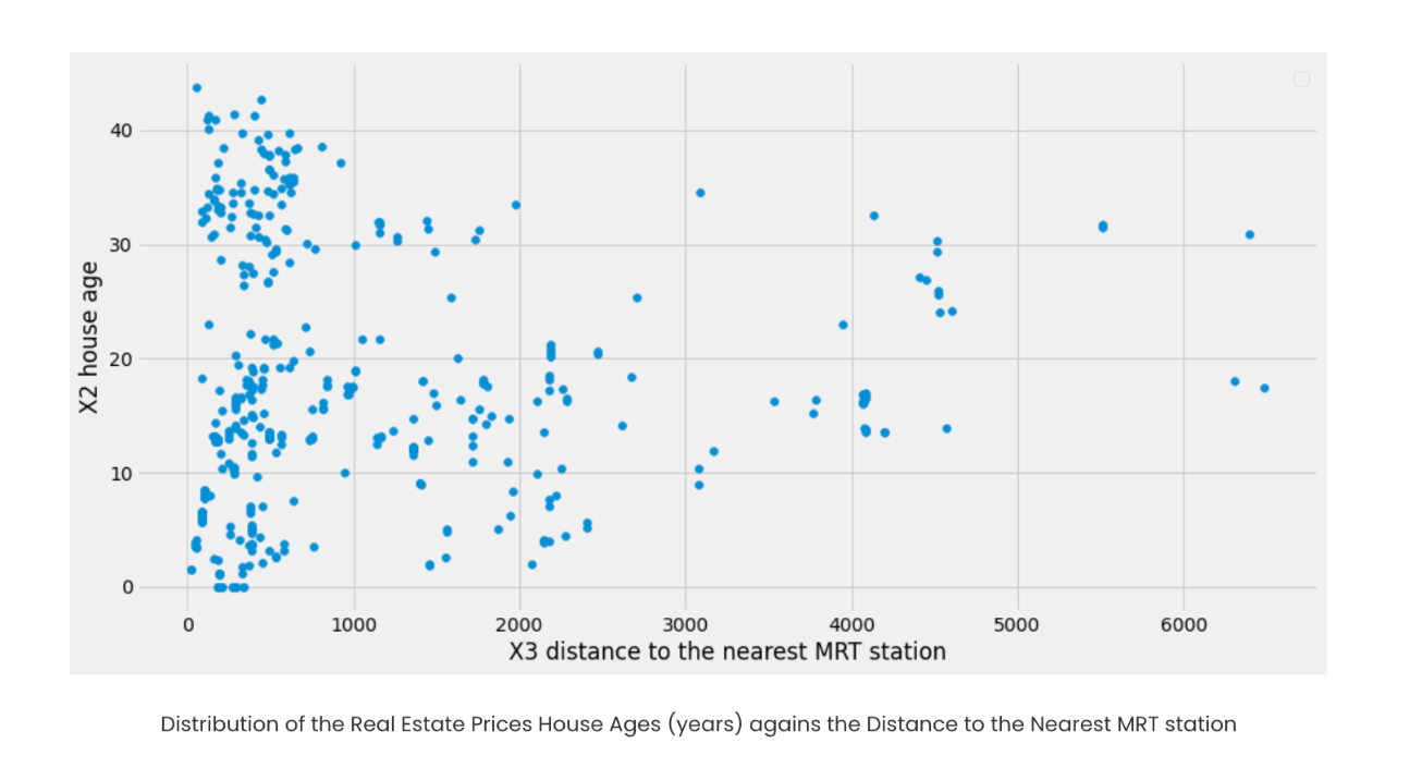
Since the data points aren’t well separated for a clear hyperplane, we’ll use K-Means clustering to organize them better. Before clustering, we’ll determine the ideal number of clusters using the Silhouette Coefficient; higher scores indicate well-separated, clearly defined clusters, while lower or negative scores suggest poor or incorrect grouping. We’ll first calculate the Silhouette Coefficient for our dataset, then split the data into train and test sets, with clustering applied on the training data as we move toward our final goal.

from sklearn.model_selection import train_test_split
from sklearn.cluster import KMeans
from sklearn.metrics import silhouette_score
import statistics
from scipy import stats

X_train, X_test, Y_train, Y_test = train_test_split(
 X, Y, test_size=0.30, random_state=42)

silhouette_coefficients = []

kmeans_kwargs= {
    "init":"random",
    "n_init":10,
    "max_iter":300,
    "random_state":42
}

for k in range(2, 11):
    kmeans = KMeans(n_clusters=k, **kmeans_kwargs)
    kmeans.fit(X_train)
    score = silhouette_score(X_train, kmeans.labels_)
    silhouette_coefficients.append(score)
    
# Plotting graph to choose the best number of clusters
# with the most Silhouette Coefficient score

import matplotlib.pyplot as plt

plt.style.use("fivethirtyeight")
plt.plot(range(2, 11), silhouette_coefficients)
plt.xticks(range(2, 11))
plt.xlabel("Number of Clusters")
plt.ylabel("Silhouette Coefficient")
plt.show()

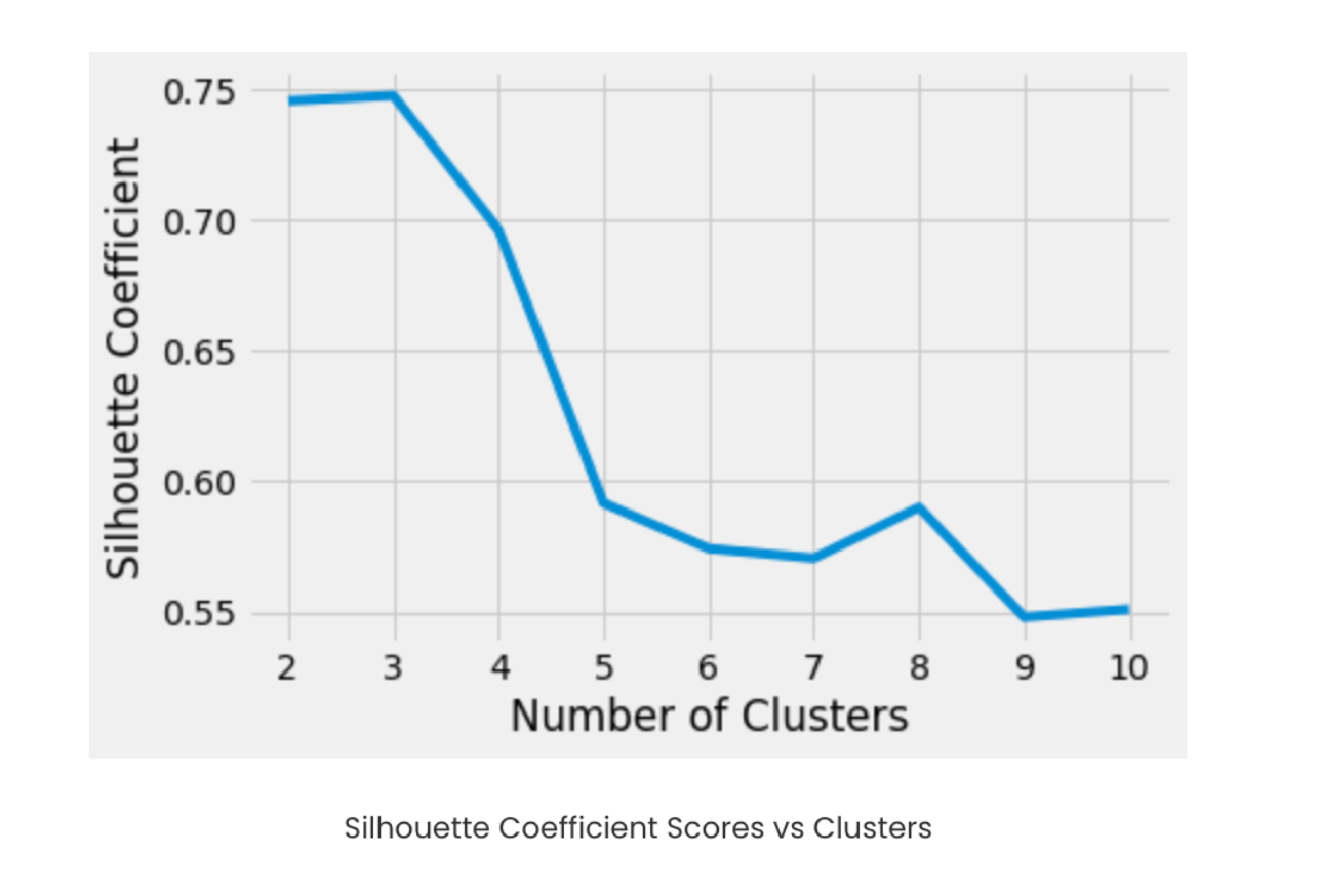
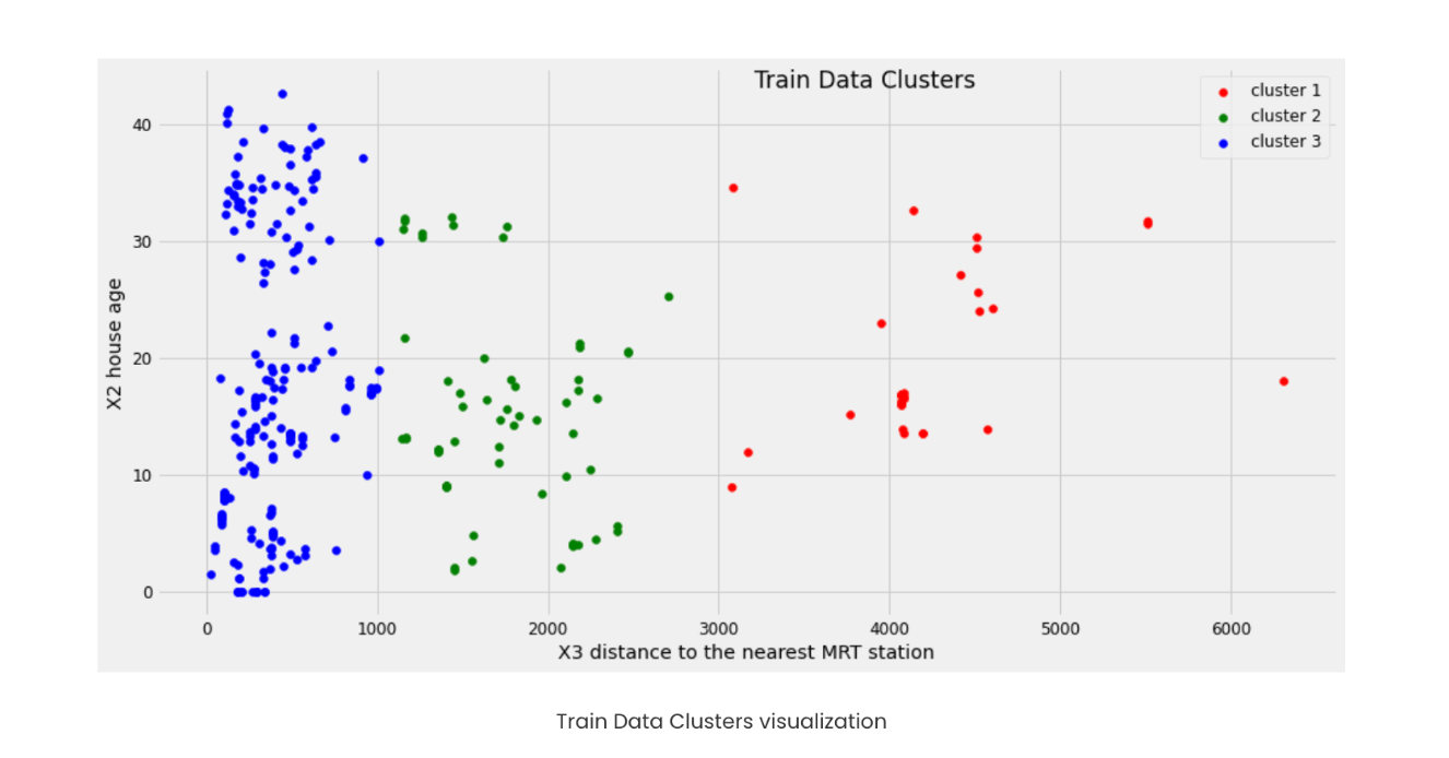
We can arrive at the conclusion that with three clusters, we can achieve better clustering. Let’s go ahead and cluster the training set data.

from sklearn.cluster import KMeans
import matplotlib.pyplot as plt
import pandas as pd # for data manipulation
import numpy as np # for data manipulation

# Instantiate the model: KMeans from sklearn
kmeans = KMeans(
    init="random",
    n_clusters=3,
    n_init=10,
    max_iter=300,
    random_state=42
)

# Fit to the training data
kmeans.fit(X_train)

train_df = pd.DataFrame(X_train,columns=['X3 distance to the nearest MRT station','X2 house age'])

# Generate out clusters
train_cluster = kmeans.predict(X_train)

# Add the target and predicted clusters to our training DataFrame
train_df.insert(2,'Y house price of unit area',Y_train) 
train_df.insert(3,'cluster',train_cluster) 
n_clusters=3
train_clusters_df = []
for i in range(n_clusters):
    train_clusters_df.append(train_df[train_df['cluster']==i])
    
colors = ['red','green','blue']
plt.rcParams['figure.figsize'] = [14, 7]
plt.rc('font', size=12)

# Plot X_train again with features labeled by cluster
for i in range(n_clusters):
  subset = []
  for count,row in enumerate(X_train):
      if(train_cluster[count]==i):
        subset.append(row)

  x = [row[0] for row in subset]
  y = [row[1] for row in subset]
  plt.scatter(x,y,c=colors[i],label="cluster "+ str(i+1))
plt.title("Train Data Clusters", x=0.6, y=0.95)
plt.xlabel("X3 distance to the nearest MRT station")
plt.ylabel("X2 house age")
plt.legend()
plt.show()

Building SVR for clusters

Now, let us go ahead and build SVR Models for each cluster. We are not focusing on the hypertuning of SVRs here. It can be done if needed by trying out various combinations of parameter values using a grid search.

import pandas as pd
import numpy as np
from sklearn.svm import SVR

n_clusters=3
cluster_svr = []
model = SVR(kernel='rbf', C=1000, epsilon=1)

for i in range(n_clusters):
    cluster_X = np.array((train_clusters_df[i])[['X3 distance to the nearest MRT station','X2 house age']])
    cluster_Y = (train_clusters_df[i])['Y house price of unit area'].values
    cluster_svr.append(model.fit(cluster_X, cluster_Y))

Let us define a function that will predict House Price (Y) by predicting the cluster first, and then the value with the corresponding SVR.

def regression_function(arr, kmeans, cluster_svr):
    result = []
    clusters_pred = kmeans.predict(arr)
    for i,data in enumerate(arr):
        result.append(((cluster_svr[clusters_pred[i]]).predict([data]))[0])
    return result,clusters

Now that we have built our end-to-end flow for prediction and constructed the required models, we can go ahead and try this out on our test data. Let us first visualize the clusters of test data with the K-means cluster we built, and then find the Y value using the corresponding SVR using the function we have written above.

from sklearn.cluster import KMeans
import matplotlib.pyplot as plt

# calculating Y value and cluster
Y_svr_k_means_pred, Y_clusters = regression_function(X_test, kmeans, cluster_svr)
    
colors = ['red','green','blue']
plt.rcParams['figure.figsize'] = [14, 7]
plt.rc('font', size=12)

n_clusters=3

# Apply our model to clustering the remaining test set for validation

for i in range(n_clusters):
  subset = []
  for count,row in enumerate(X_test):
      if(Y_clusters[count]==i):
        subset.append(row)

  x = [row[0] for row in subset]
  y = [row[1] for row in subset]
plt.scatter(x,y,c=colors[i],label="cluster "+ str(i+1))
plt.title("Test Data Clusters", x=0.6, y=0.95)
plt.xlabel("X3 distance to the nearest MRT station")
plt.ylabel("X2 house age")
plt.legend()
plt.show()

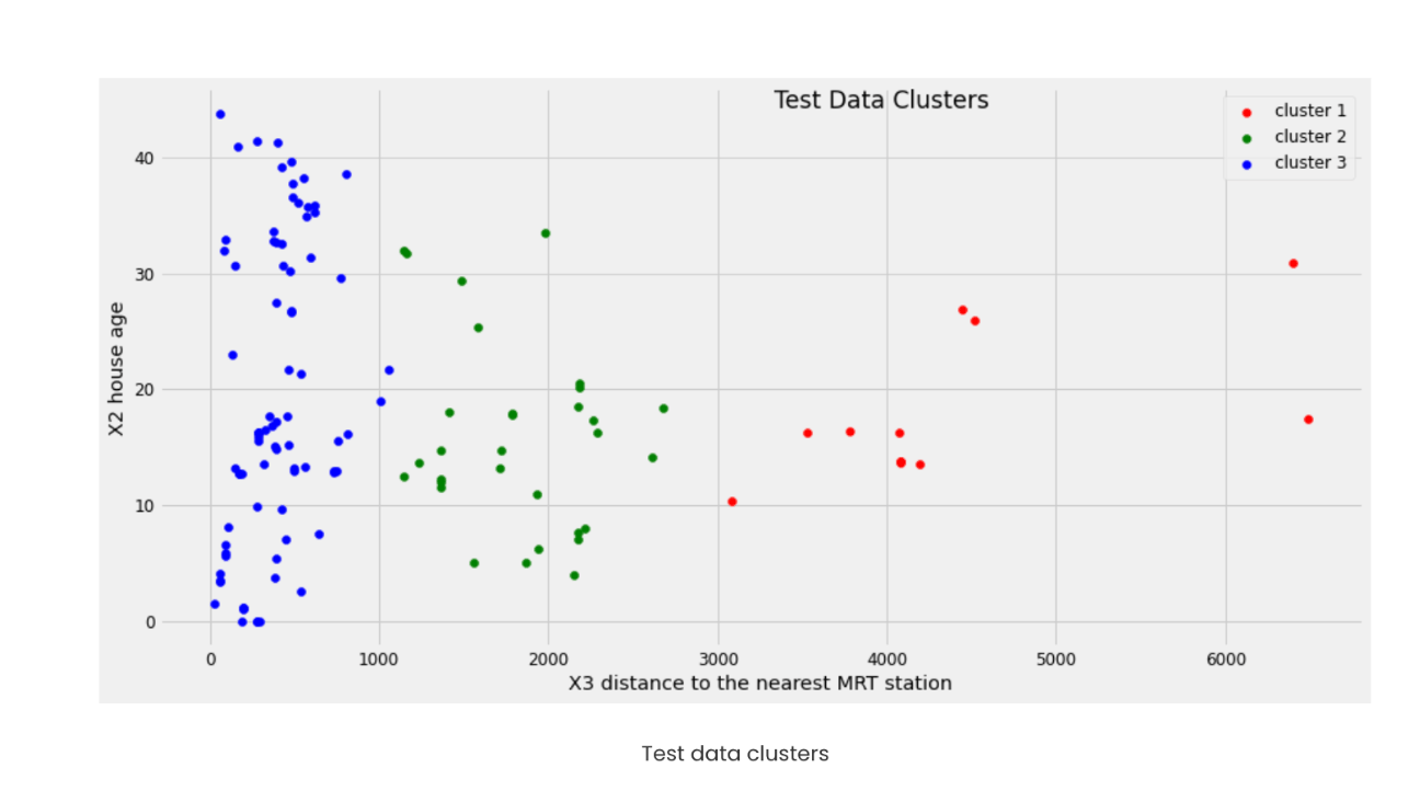
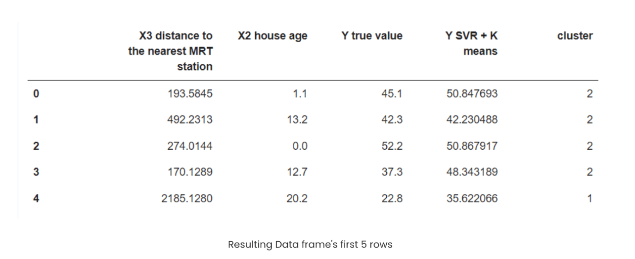
We can clearly see that we have definite clusters for test data, and we also got the Y value and have been stored in Y_svr_k_means_pred. Let us store the results and data into a data frame along with the cluster.

import pandas as pd

result_df = pd.DataFrame(X_test,columns=['X3 distance to the nearest MRT station','X2 house age'])
result_df['Y true value'] =  Y_test
result_df['Y SVR + K means'] = Y_svr_k_means_pred
result_df['cluster'] = Y_clusters
result_df.head()

Some of the results turned out very well, while others were still noticeably better than what a standalone Linear Regression or SVR model could achieve. This example demonstrates how combining K-Means and SVR can be useful, especially when data points are poorly distributed and can benefit from cluster-based modeling. In our case, we used only two independent variables; as the number of features grows, so does the complexity. In such scenarios, this hybrid approach can be even more valuable compared to traditional algorithms.

Our workflow was straightforward: start by visualizing the data to check whether clustering might help. Then, apply K-Means clustering to the training set, tuning the number of clusters using the Silhouette Coefficient to find the optimal configuration. Once clustered, we train a separate SVR model for each cluster. The final prediction pipeline works in two steps: first, identify the cluster a new data point belongs to, and then use that cluster’s SVR model to predict the target variable (Y).

• 1. Why combine K-Means and SVR instead of using SVR alone? SVR works well when data follows a consistent pattern, but if data points are unevenly distributed or form natural groups, SVR may struggle to capture those variations. K-Means helps uncover these clusters, allowing SVR to model each group more accurately.

• 2. When does this hybrid approach perform best? It works best when the dataset isn’t uniformly distributed and shows distinct patterns or subgroups. If the data is already well-structured and linearly separable, simpler models may be sufficient.

• 3. What does the Silhouette Coefficient tell us? The Silhouette Score measures how well data points fit within their assigned clusters. A higher score indicates that the clusters are well separated and meaningful, helping determine the best number of clusters for K-Means.

• 4. Do I need to train multiple SVR models? Yes. Each cluster gets its own SVR model. During prediction, the model first identifies the cluster of the new data point and then uses the corresponding SVR model to predict the target value.

• 5. Is this method suitable for high-dimensional data? It can be, but complexity increases significantly as the number of features grows. Clustering becomes harder, and the computational cost rises. However, if the data genuinely benefits from cluster-level modeling, the performance gains can justify the effort.

• 6. Can this approach replace other regression algorithms entirely? Not necessarily. It’s most effective for datasets with cluster-like structures. For simpler, well-behaved datasets, traditional regression or SVR alone may be more efficient.

Regression is one of the straightforward tasks carried out in Machine Learning. Still, it can become increasingly difficult to find the right algorithm that can build a model with decent accuracy for deploying to production. It is always better to try most of the algorithms out there before finalizing one. There may be instances where a simple linear regression would have worked wonders instead of the huge random forest regression. Having a solid understanding of the data and its nature will help us choose algorithms easily, and visualization also helps in the process.

This article focuses on exploring the possibility of the combination of K-Means clustering and Support Vector Regression. This approach won’t always suit all cases of regression, as it stresses the clustering possibility. One good example of such a problem can be soil moisture prediction, as it may vary with seasons and a lot of cyclic features, resulting in clustered data points.

K-Means clustering saves us from manual decisions on clusters, and SVR handles non-linearity very well. Both SVR and K-Means alone have a lot more in-depth to explore, including Kernels, centroid initialization, and the list goes on, so I highly encourage you to read more on the topics to yield a better model. Thanks for reading!

• Scikit-learn: A Beginner’s Guide to Machine Learning in Python
• What is Linear Regression in Machine Learning?
• Regression vs Transformers: Key Differences and When to Use Each Model
• Mastering Logistic Regression with Scikit-Learn: A Complete Guide
• Principal Component Analysis (PCA) in Machine Learning
• Decision Trees Made Simple: Machine Learning Explained
• A Practical Guide to Random Forests in Machine Learning