By Shaoni Mukherjee and samuel ozechi

Introduction
Model ensembling is a popular approach in machine learning that helps improve how well models perform, especially on new, unseen data. At its core, it’s about combining the strengths of multiple models to get better results than any single model could on its own. This technique boosts accuracy, increases robustness, and enhances the model’s ability to generalize.
Tree-based algorithms, for example, often shine in certain tasks because they naturally work by combining the outputs of multiple decision trees to create a stronger overall prediction.
There are different ways to combine models in an ensemble, ranging from simple methods like averaging their predictions to more sophisticated techniques like bagging, boosting, or stacking. Each method offers its own way of blending the models to make the final decision more reliable.
Key Takeaways
-
Ensemble learning combines multiple neural networks to improve prediction accuracy, robustness, and generalization.
-
The workflow typically involves preparing the dataset, training multiple models, and integrating their outputs using ensemble strategies.
-
Common ensemble methods include:
- Concatenation Ensemble: Merges features from multiple models for a richer representation.
- Average Ensemble: Takes the average of predictions from all models, simple yet effective.
- Weighted Average Ensemble: Assigns different importance (weights) to models based on their individual performance.
-
A comparison between single and ensemble models shows that ensembles often outperform single models in complex tasks but may introduce more computational overhead.
-
Ensemble methods are particularly beneficial when individual models make diverse errors that can be corrected collectively.
-
Choosing the right ensemble technique depends on your data type, model architecture, and evaluation goals.
In contrast to classical algorithms, it’s not common for multiple neural network models to be ensembled for a single task. This is mostly because single models are often enough to map the relationship between features and targets, and ensembling multiple neural networks might complicate the model for smaller tasks and lead to overfitting. It’s most common for practitioners to increase the size of a single neural network model to properly fit the data rather than ensemble multiple neural network models into one.
However, for larger tasks, ensembling multiple neural networks, especially ones trained on similar problems, could prove quite useful and improve the performance of the final model and its ability to generalize to broader use cases.
Oftentimes, there is a need to try out multiple models with different configurations to select the best-performing model for a problem. Neural network ensembling offers the option of utilizing the information of the different models to develop a more balanced and efficient model.
For example, combining multiple network models that were trained on a particular dataset (such as the Imagenet dataset) could prove useful to improve the performance of a model being trained on a dataset with similar classes. The different information learned by the models could be combined through model ensembling to improve the model’s overall performance and robustness of an aggregated model. Before ensembling such models, it is important to train and fine-tune the ensemble members to ensure that each model contributes relevant information to the final model.
The Dataset
For this tutorial, we will use image classification of natural images. We will use the Natural Images Dataset, which contains 6899 images of natural images representing 8 classes. The classes represented in the dataset are aeroplane, car, cat, dog, fruit, motorbike, and person.
Our aim is to develop a neural network model capable of identifying images belonging to different classes and accurately classifying new images of each class.
Workflow
We would develop three different models for our task and then ensemble using different methods. It is important to configure our models to provide relevant information to our final model.
Set Seed for Reproducibility and Preview Sample Images per Class
# Seed environment
seed_value = 1 # seed value

# Set`PYTHONHASHSEED` environment variable at a fixed value
import os os.environ['PYTHONHASHSEED']=str(seed_value)
rti
# Set the `python` built-in pseudo-random generator at a fixed value
import random
random.seed = seed_value

# Set the `numpy` pseudo-random generator at a fixed value
import numpy as np
np.random.seed = seed_value

# Set the `tensorflow` pseudo-random generator at a fixed value import tensorflow as tf tf.seed = seed_value
Set the data configurations and get the classes
# set configs
base_path = './natural_images'
target_size = (224,224,3)

# define shape for all images # get classes classes = os.listdir(base_path) print(classes)

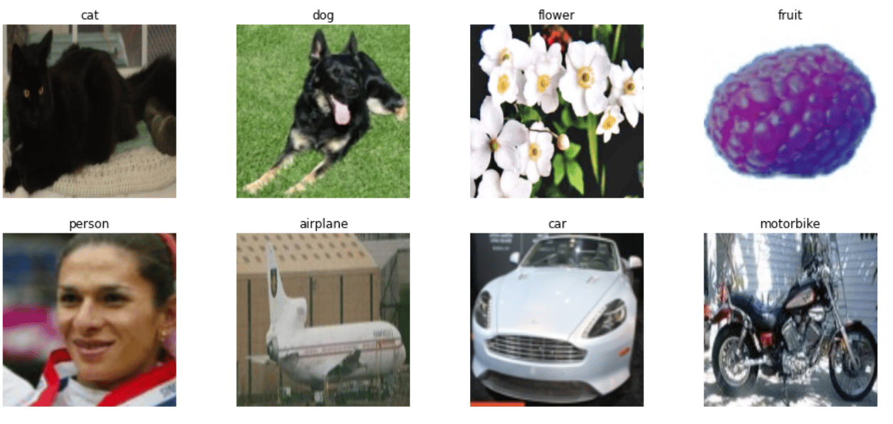
Plot Sample images of the dataset
# plot sample images

import matplotlib.pyplot as plt
import cv2

f, axes = plt.subplots(2, 4, sharex=True, sharey=True, figsize = (16,7))

for ax, label in zip(axes.ravel(), classes):
    img = np.random.choice(os.listdir(os.path.join(base_path, label)))
    img = cv2.imread(os.path.join(base_path, label, img))
    img = cv2.resize(img, target_size[:2])
    ax.imshow(cv2.cvtColor(img, cv2.COLOR_BGRA2RGB))
    ax.set_title(label)
    ax.axis(False)
Load the images
We load the images in batches using the Keras Image Generator and specify a validation split to split the dataset into training and validation splits.
We also apply random image augmentation to expand the training dataset, improving the model’s performance and generalization ability.
from keras.preprocessing.image import ImageDataGenerator

batch_size = 32

datagen = ImageDataGenerator(rescale=1./255,
                                   rotation_range=20,
                                   shear_range=0.2,
                                   zoom_range=0.2,
                                   width_shift_range = 0.2,
                                   height_shift_range = 0.2,
                                   vertical_flip = True,
                                   validation_split=0.25)
train_gen = datagen.flow_from_directory(base_path,
                                               target_size=target_size[:2],
                                               batch_size=batch_size,
                                               class_mode='categorical',
                                               subset='training')
val_gen =  datagen.flow_from_directory(base_path,
                                               target_size=target_size[:2],
                                               batch_size=batch_size,
                                               class_mode='categorical',
                                               subset='validation',
                                               shuffle=False)
1. Build and train a custom model
For our first model, we built a custom model using the Tensorflow functional method.
# Build model
input = Input(shape= target_size)

x = Conv2D(filters=32, kernel_size=(3,3), activation='relu')(input)
x = MaxPool2D(2,2)(x)

x = Conv2D(filters=64, kernel_size=(3,3), activation='relu')(x)
x = MaxPool2D(2,2)(x)

x = Conv2D(filters=128, kernel_size=(3,3), activation='relu')(x)
x = MaxPool2D(2,2)(x)

x = Conv2D(filters=256, kernel_size=(3,3), activation='relu')(x)
x = MaxPool2D(2,2)(x)

x = Dropout(0.25)(x)
x = Flatten()(x)
x = Dense(units=128, activation='relu')(x)
x = Dense(units=64, activation='relu')(x)
output = Dense(units=8, activation='softmax')(x)

custom_model  = Model(input, output, name= 'Custom_Model')
Next, we compile the custom model and set up callbacks to manage training. We use learning rate reduction on plateau, EarlyStopping to halt training when no further improvement is observed, and ModelCheckpoint to save the best model at each epoch. These are standard practices for effective deep learning training.
# compile model
custom_model.compile(loss= 'categorical_crossentropy', optimizer='rmsprop', metrics=['accuracy'])

# initialize callbacks
reduceLR = ReduceLROnPlateau(monitor='val_loss', patience= 3, verbose= 1,                                  mode='min', factor=  0.2, min_lr = 1e-6)

early_stopping = EarlyStopping(monitor='val_loss', patience = 5 , verbose=1,                                  mode='min', restore_best_weights= True)

checkpoint = ModelCheckpoint('CustomModel.weights.hdf5', monitor='val_loss',                               verbose=1,save_best_only=True, mode= 'min')

callbacks= [reduceLR, early_stopping,checkpoint]
Now we can define our training configurations and train our custom model.
# define training config
TRAIN_STEPS = 5177 // batch_size
VAL_STEPS = 1722 //batch_size
epochs = 80

# train model
custom_model.fit(train_gen, steps_per_epoch= TRAIN_STEPS, validation_data=val_gen, validation_steps=VAL_STEPS, epochs= epochs, callbacks= callbacks)
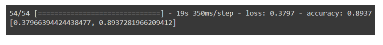
After training our custom model, we can evaluate its performance. I will evaluate the model on the validation set. In practice, it is preferable to set aside a separate test set for model evaluation.
# Evaluate the model
custom_model.evaluate(val_gen)
Validation loss and accuracy
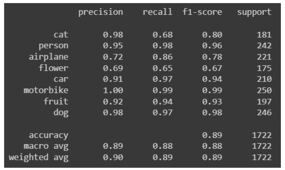
We can also retrieve the prediction and actual validation labels so as to check the classification report and confusion matrix evaluations for the custom model.
# get validation labels
val_labels = []
for i in range(VAL_STEPS + 1):
  val_labels.extend(val_gen[i][1])

val_labels = np.argmax(val_labels, axis=1)
# show classification report
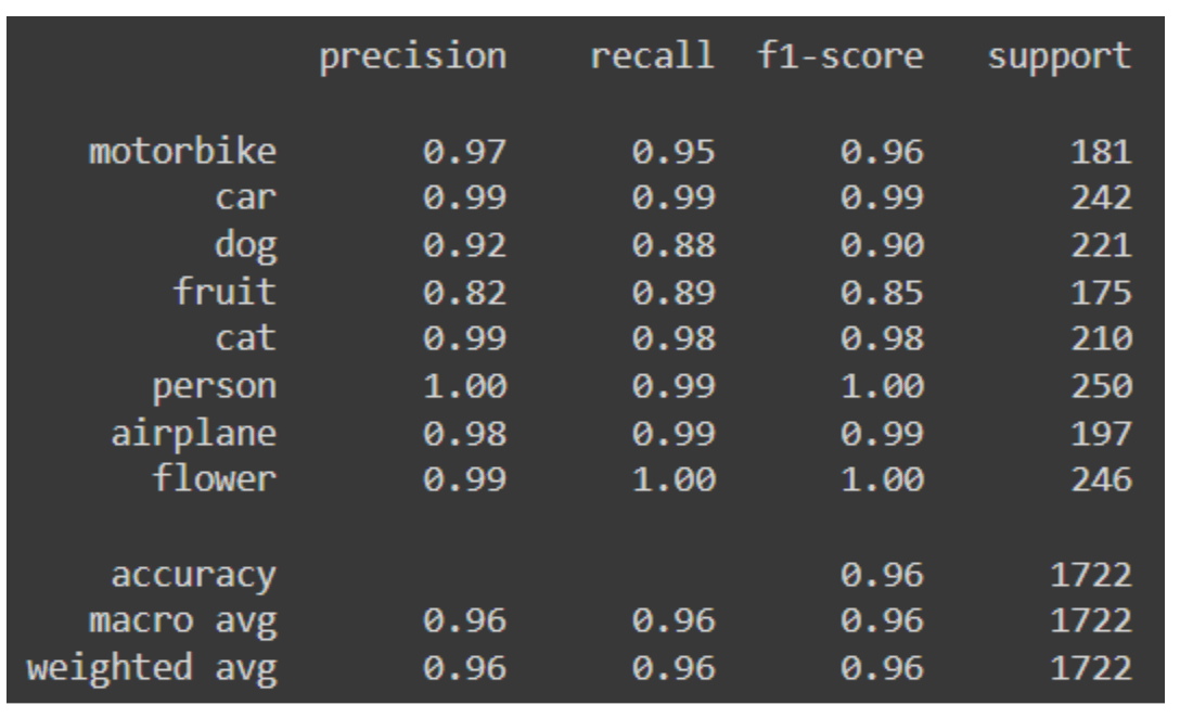
from sklearn.metrics import classification_report
print(classification_report(val_labels, predicted_labels, target_names=classes))
Classification Report
# function to plot confusion matrix

import itertools

def plot_confusion_matrix(actual, predicted):

    cm = confusion_matrix(actual, predicted)
    cm = cm.astype('float') / cm.sum(axis=1)[:, np.newaxis]

    plt.figure(figsize=(7,7))
    cmap=plt.cm.Blues
    plt.imshow(cm, interpolation='nearest', cmap=cmap)
    plt.title('Confusion matrix', fontsize=25)

    tick_marks = np.arange(len(classes))
    plt.xticks(tick_marks, classes, rotation=90, fontsize=15)
    plt.yticks(tick_marks, classes, fontsize=15)

    thresh = cm.max() / 2.
    for i, j in itertools.product(range(cm.shape[0]), range(cm.shape[1])):
        plt.text(j, i, format(cm[i, j], '.2f'),
        horizontalalignment="center",
        color="white" if cm[i, j] > thresh else "black", fontsize = 14)

    plt.ylabel('True label', fontsize=20)
    plt.xlabel('Predicted label', fontsize=20)
    plt.show()
# plot confusion matrix
plot_confusion_matrix(val_labels, predicted_labels)
Confusion Matrix using the Custom Model
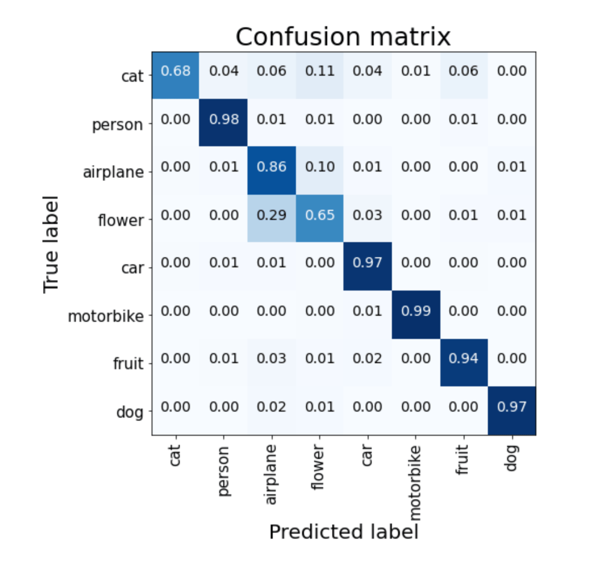
From the model evaluation, we notice that the custom model could not properly identify the images of cats and flowers. It also gives sub-optimal precision for identifying aeroplanes.
Next, we would try out a different model-building technique: using weights learned by networks pre-trained on the Imagenet dataset to boost our model’s performance in classes with lower accuracy scores.
2. Using a pre-trained VGG16 model.
For our second model, we would be using the VGG16 model pre-trained on the Imagenet dataset to train a model for our use case. This allows us to inherit the weights learned from training on a similar dataset to boost our model’s performance.
Initializing and fine-tuning the VGG16 model
# Import the VGG16 pretrained model
from tensorflow.keras.applications import VGG16

# initialize the model vgg16 = VGG16(input_shape=(224,224,3), weights='imagenet', include_top=False)

# Freeze all but the last 3 layers for layer in vgg16.layers[:-3]: layer.trainable = False

# build model
input = vgg16.layers[-1].output # input is the last output from vgg16

x = Dropout(0.25)(input)
x = Flatten()(x)
output = Dense(8, activation='softmax')(x)

# create the model
vgg16_model = Model(vgg16.input, output, name='VGG16_Model')
We initialize the pre-trained model and freeze all but the last three layers so we can utilize the weights of the models and learn new information in the last 3 layers that are specific to our use case. We also add a dropout layer to regularize the model from overfitting on our dataset before adding our final output layer.
We can then train our VGG16 fine-tuned model using similar training configurations to our custom model.
# compile the model
vgg16_model.compile(optimizer= SGD(learning_rate=1e-3), loss= 'categorical_crossentropy', metrics= ['accuracy'])

# reinitialize callbacks
checkpoint = ModelCheckpoint('VggModel.weights.hdf5', monitor='val_loss', verbose=1,save_best_only=True, mode= 'min')

callbacks= [reduceLR, early_stopping,checkpoint]

# Train model
vgg16_model.fit(train_gen, steps_per_epoch= TRAIN_STEPS, validation_data=val_gen, validation_steps=VAL_STEPS, epochs= epochs, callbacks= callbacks)
After training, we can evaluate the model’s performance using similar scripts from the last model evaluation.
# Evaluate the model
vgg16_model.evaluate(val_gen)

# get the model predictions
predicted_labels = np.argmax(vgg16_model.predict(val_gen), axis=1)

# show classification report
print(classification_report(val_labels, predicted_labels, target_names=classes))

# plot confusion matrix
plot_confusion_matrix(val_labels, predicted_labels)

Classification report using the pre-trained VGG model
Confusion Matrix report using the pre-trained VGG model
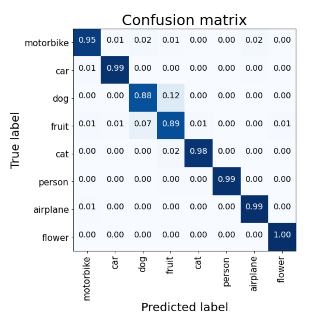
Using a pre-trained VGG16 model produced better performance, especially for the classes with lower scores.
Finally, before ensembling, we would use another pre-trained model with much fewer parameters than the VGG16. The aim is to utilize different architectures so we can benefit from their varying properties to improve the quality of our final model. We would be using the Mobilenet model pre-trained on the same Imagenet dataset.
3. Using a pre-trained Mobilenet model.
For our final model, we would be fine-tuning the MobileNet model
# initializing the mobilenet model
mobilenet = MobileNet(input_shape=(224,224,3), weights='imagenet', include_top=False)

# freezing all but the last 5 layers
for layer in mobilenet.layers[:-5]:
  layer.trainable = False

# add few mor layers
x = mobilenet.layers[-1].output
x = Dropout(0.5)(x)
x = Flatten()(x)
x = Dense(32, activation='relu')(x)
x = Dropout(0.5)(x)
x = Dense(16, activation='relu')(x)
output = Dense(8, activation='softmax')(x)

# Create the model
mobilenet_model = Model(mobilenet.input, output, name= "Mobilenet_Model")
For training the model, we maintain some of the previous configurations from our previous training.
# compile the model
mobilenet_model.compile(optimizer= SGD(learning_rate=1e-3), loss= 'categorical_crossentropy', metrics= ['accuracy'])

# reinitialize callbacks
checkpoint = ModelCheckpoint('MobilenetModel.weights.hdf5', monitor='val_loss', verbose=1,save_best_only=True, mode= 'min')

callbacks= [reduceLR, early_stopping,checkpoint]

# model training
mobilenet_model.fit(train_gen, steps_per_epoch= TRAIN_STEPS, validation_data=val_gen, validation_steps=VAL_STEPS, epochs=epochs, callbacks= callbacks)
After training our fine-tuned Mobilenet model, we can then evaluate its performance.
# Evaluate the model
mobilenet_model.evaluate(val_gen)

# get the model's predictions
predicted_labels = np.argmax(mobilenet_model.predict(val_gen), axis=1)

# show the classification report
print(classification_report(val_labels, predicted_labels, target_names=classes))

# plot the confusion matrix
plot_confusion_matrix(val_labels, predicted_labels)

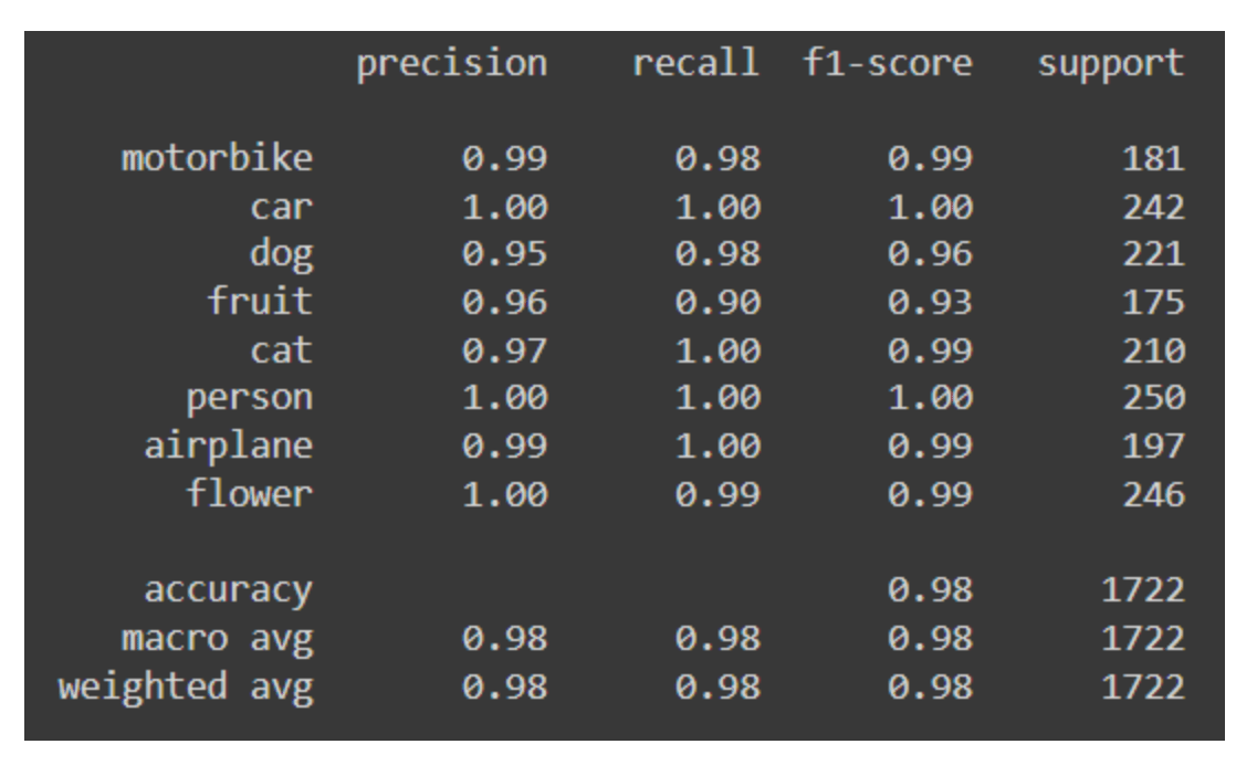
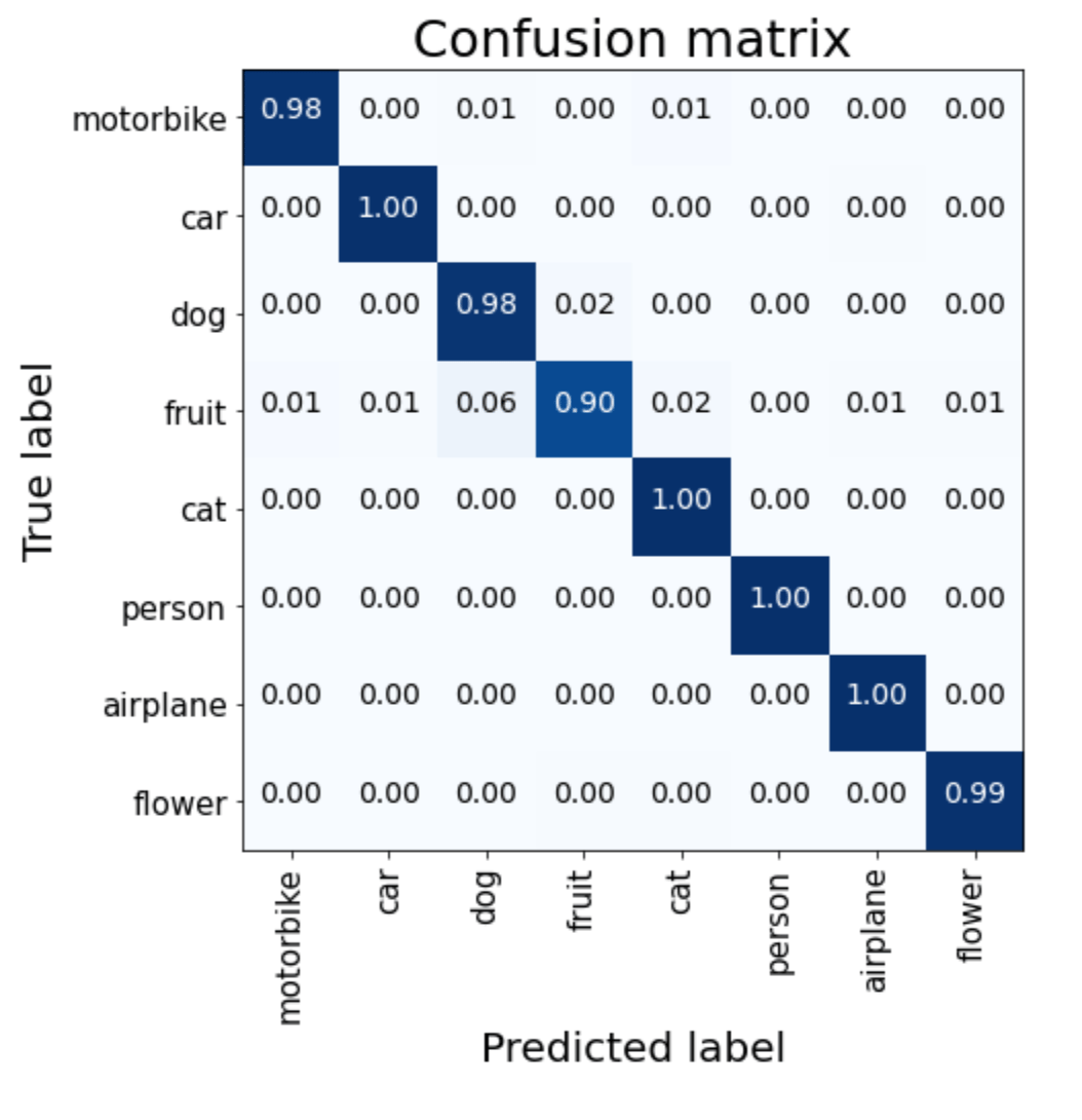
The fine-tuned Mobilenet model performs better than the previous models and notably improves the identification of dogs and flowers.
While it would be fine to use the trained Mobilenet model or any of our models as our final choice, combining the structure and weights of the three models might prove better in developing a single, more generalizable model in production.
Ensembling The Models
As earlier stated, we would use three different ensembling methods to ensemble the models: Concatenation, Average, and Weighted Average.
The methods have their pros and cons, which are often considered to determine the choice for a particular use case.
Concatenation Ensemble
This involves merging the parameters of multiple models into a single model. This is made possible in Tensorflow by the concatenation layer which receives inputs of tensors of the same shape (except for the concatenation axis) and merges them into one. This layer can therefore be used to merge all the information learnt by the different models side by side on a single axis into a single model.
To merge our models, we would simply input our models into the concatenation layer.
# concatenate the models

# import concatenate layer
from tensorflow.keras.layers import Concatenate

# get list of models
models = [custom_model, vgg16_model, mobilenet_model]

input = Input(shape=(224, 224, 3), name='input') # input layer

# get output for each model input
outputs = [model(input) for model in models]

# contenate the ouputs
x = Concatenate()(outputs)

# add further layers
x = Dropout(0.5)(x)
output = Dense(8, activation='softmax', name='output')(x) # output layer

# create concatenated model
conc_model = Model(input, output, name= 'Concatenated_Model')
After concatenation, we added further layers as deemed appropriate for our task. In this example, I have added a dropout layer and a final output layer with the appropriate output dimensions of our use case.
Let’s check the structure of our concatenated model.
# show model structure
from tensorflow.keras.utils import plot_model
plot_model(conc_model)
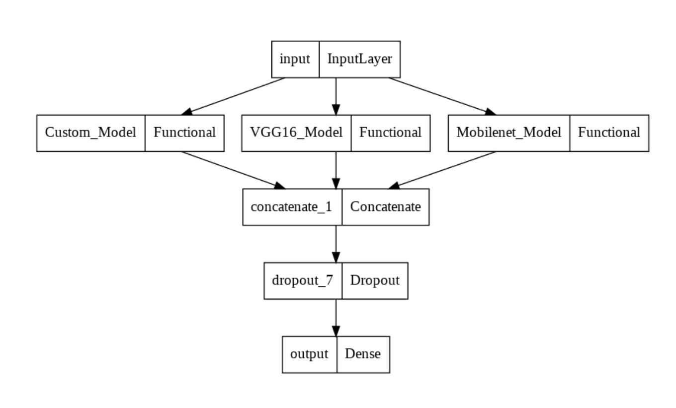
Structure of the Concatenated Model
We can see how the three different functional models we’ve built are merged into one with further dropout and output layers.
This could prove useful in certain cases as we are utilizing all the information gained by the different models. The problem with this method is that the dimension of our final model is a concatenation of the dimensions of all the ensemble members, which could lead to a dimensionality explosion, the inclusion of irrelevant information, and consequently, overfitting.
Average Ensemble
Rather than risk exploding the model’s dimension and overfitting for simpler tasks by concatenating multiple models, we could simply make our final model the average of all our models. This way, we are able to maintain a reasonable average dimension for our final model while utilizing the information of all our models.
This time we will use the Tensorflow Average layer, which receives inputs and outputs their average. Therefore, our final model is an average of the parameters of our input models.
To ensemble our model by average, we simply combine our models at the average layer.
# average ensemble model

# import Average layer
from tensorflow.keras.layers import Average

input = Input(shape=(224, 224, 3), name='input')  # input layer

# get output for each input model
outputs = [model(input) for model in models]

# take average of the outputs
x = Average()(outputs)

x = Dense(16, activation='relu')(x)
x = Dropout(0.3)(x)
output = Dense(8, activation='softmax', name='output')(x) # output layer

# create average ensembled model
avg_model = Model(input, output)
As previously seen, further layers can be added to the network as deemed fit. We can also see the structure of the Average ensembled model.
# show model structure
plot_model(avg_model)
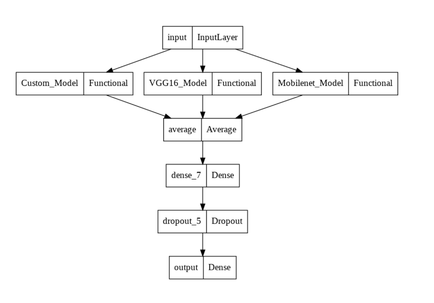
This approach to ensembling is particularly useful because, by taking an average, models with lower performance for certain classes are boosted by models with higher performance for such classes, thereby improving the model’s overall performance and generalization.
The downside to this approach is that by taking the average, certain information from the models would not be included in the final model. Another is that because we are taking a simple average, the superiority and relevance of certain models are lost. As in our use case, the superiority in performance of the Mobilenet Model over other models is lost.
This could be resolved by taking a weighted average of the models when ensembling, such that it reflects the importance of each model to the final decision.
Weighted Average Ensemble
In weighted average ensembling, the outputs of the models are multiplied by an assigned weight, and an average is taken to get a final model. By assigning weights to the models when ensembling this way, we preserve their importance and contribution to the final decision.
While TensorFlow does not have a built-in layer for weighted average ensembling, we could utilize attributes of the built-in Layer class to implement a custom weighted average ensemble layer. For a weighted average ensemble, it is necessary that the weights sum up to one, we can ensure this by applying a softmax function on the weights before ensembling. You can see more about creating custom layers in TensorFlow here.
Implementing a custom weighted average layer
First, we define a custom function to set our weights.
# function for setting weights

import numpy as np

def weight_init(shape =(1,1,3), weights=[1,2,3], dtype=tf.float32):
    return tf.constant(np.array(weights).reshape(shape), dtype=dtype)
Here, we have set our models’ weights to 1, 2, and 3, respectively. We can then build our custom weighted average layer.
# implement custom weighted average layer

import tensorflow as tf
from tensorflow.keras.layers import Layer, Concatenate

class WeightedAverage(Layer):

    def __init__(self):
        super(WeightedAverage, self).__init__()

    def build(self, input_shape):

        self.W = self.add_weight(
                    shape=(1,1,len(input_shape)),
                    initializer=weighted_init,
                    dtype=tf.float32,
                    trainable=True)
    def call(self, inputs):

        inputs = [tf.expand_dims(i, -1) for i in inputs]
        inputs = Concatenate(axis=-1)(inputs)
        weights = tf.nn.softmax(self.W, axis=-1)

        return tf.reduce_mean(weights*inputs, axis=-1)
To build our custom weighted average layer, we inherited attributes of the built-in Layer class and added weights using our weights initialization function. We apply a softmax to our initialized weights so that they sum up to one before multiplying them by the models. Finally, we get the mean reduction of the weighted inputs to get our final model.
We can then ensemble our model using the custom weighted average layer.
input = Input(shape=(224, 224, 3), name='input')  # input layer

# get output for each input model
outputs = [model(input) for model in models]

# get weighted average of outputs
x = WeightedAverage()(outputs)

output = Dense(8, activation='softmax')(x) # output layer

weighted_avg_model = Model(input, output, name= 'Weighted_AVerage_Model')
Let’s check the structure of our weighted average model.
# plot model
plot_model(weighted_avg_model)
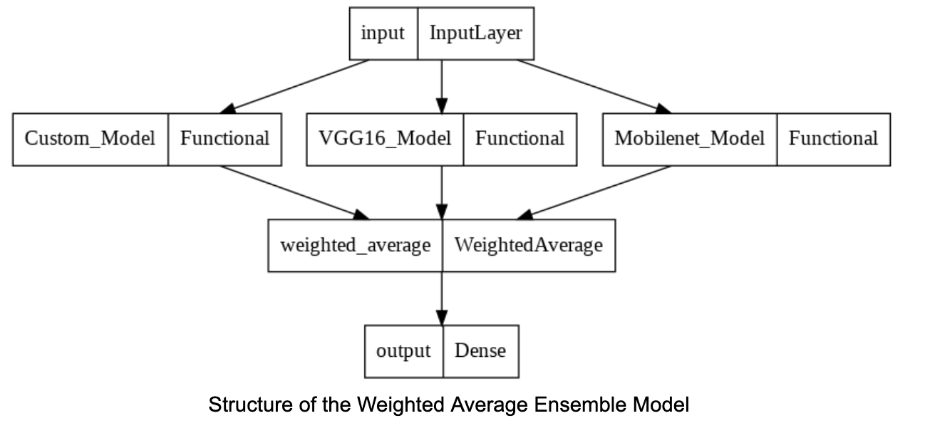
Structure of the Weighted Average Ensemble Model As in the previous methods, our models are ensembled, but this time, as a weighted average of the three models. The output dimension of the ensembled model is also compatible with the required output dimension for our task without adding any further layers.
Also, rather than manually setting our weights using a custom weight initializing function, we could utilize Tensorflow’s built-in weight initializers to initialize weights that are optimized during training. See here for the available built-in weight initializers in Tensorflow.
Single Model vs Ensemble
| Metric | Single Model | Ensemble (Stacking) |
|---|---|---|
| Accuracy | ~85% | ~89–91% |
| Training Time | Low | High (Multiple Models) |
| Inference Time | Fast | Slower (Multiple Passes) |
| Generalization | Moderate | High |
| Robustness | Lower | Higher |
Ensembling improves accuracy and robustness but increases training/inference time and memory usage. Ensembling is useful when performance matters more than latency.
FAQ’s
1. What is ensembling with neural networks?
Ensembling with neural networks involves combining the predictions of multiple neural models to improve accuracy, robustness, and generalization on unseen data.
2. Can you ensemble different types of neural networks?
Yes, you can ensemble models like CNNs, LSTMs, and MLPs together. This is especially useful when each model captures different aspects of the data.
3. How many models should I use in an ensemble?
There’s no fixed number—it depends on your dataset, compute power, and performance goals. Even 2–3 well-chosen models can offer noticeable improvements.
4. What’s the difference between bagging and stacking?
Bagging trains models independently on different data subsets and averages predictions, while stacking combines diverse models using a meta-learner trained on their outputs.
5. How is ensembling used in LLMs?
In large language models (LLMs), ensembling is used to combine outputs from multiple model checkpoints or versions, improving accuracy and reducing bias or hallucination.
Summary
Model ensembling enhances the performance and generalization of machine learning models by combining multiple models into a unified architecture. In neural networks, TensorFlow allows for various ensembling strategies such as concatenation, averaging, and custom weighted averaging. While concatenation preserves all features (at the cost of increased dimensionality), averaging simplifies the model but may overlook model importance. Custom weighted averaging addresses this by learning optimal weights during training. These techniques can also be extended with more advanced or task-specific operations, making ensembling a flexible and powerful tool in deep learning.
Related Resources
- https://www.digitalocean.com/resources/articles/what-is-deep-learning
- https://www.digitalocean.com/community/tutorials/constructing-neural-networks-from-scratch
- https://www.digitalocean.com/community/tutorials/global-pooling-in-convolutional-neural-networks
- https://www.digitalocean.com/community/tutorials/random-forest-in-machine-learning
- https://www.digitalocean.com/community/tutorials/decision-trees-machine-learning-explained
Thanks for learning with the DigitalOcean Community. Check out our offerings for compute, storage, networking, and managed databases.
About the author(s)
With a strong background in data science and over six years of experience, I am passionate about creating in-depth content on technologies. Currently focused on AI, machine learning, and GPU computing, working on topics ranging from deep learning frameworks to optimizing GPU-based workloads.
Still looking for an answer?
This textbox defaults to using Markdown to format your answer.
You can type !ref in this text area to quickly search our full set of tutorials, documentation & marketplace offerings and insert the link!
 This work is licensed under a Creative Commons Attribution-NonCommercial- ShareAlike 4.0 International License.
Become a contributor for community
Get paid to write technical tutorials and select a tech-focused charity to receive a matching donation.

DigitalOcean Documentation
Full documentation for every DigitalOcean product.

Resources for startups and AI-native businesses
The Wave has everything you need to know about building a business, from raising funding to marketing your product.
The developer cloud
Scale up as you grow — whether you're running one virtual machine or ten thousand.

Start building today
From GPU-powered inference and Kubernetes to managed databases and storage, get everything you need to build, scale, and deploy intelligent applications.
