AI Technical Writer

Introduction
As AI adoption grows across industries, more GPUs are deployed, more training cycles run, and more servers operate around the clock. All of these contribute to the total global electricity consumption to a large extent. Modern GPUs are known to draw 300–700W each, and when used in clusters of hundreds or thousands, the total power usage increases rapidly. Also, model sizes are growing exponentially from millions → billions → trillions of parameters, and training cost grows even faster than model size. This exponential growth leads directly to exponential energy usage. This has led to increases in carbon footprint across training, inference, and overall AI deployment at scale.
This is why energy efficiency is now a critical design goal for ML systems. Organizations are no longer just optimizing models only for accuracy and speed; they’re increasingly prioritizing compute efficiency, sustainability, and operational cost reduction. One of the most effective ways to achieve all three is through precision scaling, a technique that reduces the number of bits used to represent model weights and activations.
In simple terms, precision scaling shifts models from high-precision formats like FP32 to more compact numerical representations such as FP16, INT8, and even INT4. Fewer bits mean fewer computations, less memory movement, and lower power consumption without significantly compromising performance. This approach is rapidly becoming a popular method for building energy-efficient deep learning systems at both training and inference stages.
Good-to-Know Concepts in Deep Learning
Before we start, here are a few concepts that will help you follow this article and gain a better understanding of how modern deep learning systems work.
Core Compute Concepts
- FLOPs (Floating Point Operations per Second): A measure of how many mathematical operations (like adds or multiplies) a processor can perform in one second. More FLOPs = faster compute.
- Matrix Multiplications (MatMuls): The core operation in neural networks, where two matrices are multiplied. Used in attention layers, MLPs, and convolution layers. They consume most of the training compute.
- Tensors: Multi-dimensional arrays (like vectors, matrices, or higher-dimensional blocks) that store data in deep learning models. Almost all neural network operations take tensors as input and output.
- Bits: A bit is the smallest unit of data in computing. The number of bits determines how precisely a number is stored (e.g., FP32 = 32 bits). Fewer bits → faster compute and lower memory use.
Precision & Numerical Concepts
- Mixed Precision Training: A training approach where different parts of the model use different numeric formats (e.g., FP16 for compute, FP32 for stability). It speeds up training while keeping accuracy stable.
- Low Precision Formats: FP32 (high precision), FP16/BF16 (medium precision), FP8/INT8/INT4 (ultra-low precision). Lower precision reduces compute, memory, and energy costs.
- Quantization: The process of storing and computing with lower-bit numbers. Often used during inference to reduce memory footprint and increase speed.
Performance & Efficiency Concepts
- Throughput: The number of samples, tokens, or requests a system can process per second. Higher throughput = faster model performance.
- Latency: The time taken for one input to get a response. Lower latency = quicker interaction.
- GPU Hours: A cost and efficiency metric representing how long a GPU is used. For example: 8 GPUs running for 10 hours = 80 GPU-hours.
- Memory Bandwidth: How fast data can move between GPU memory and compute units. Important because many neural workloads are memory-bound, not compute-bound.
Training Dynamics & Model Concepts
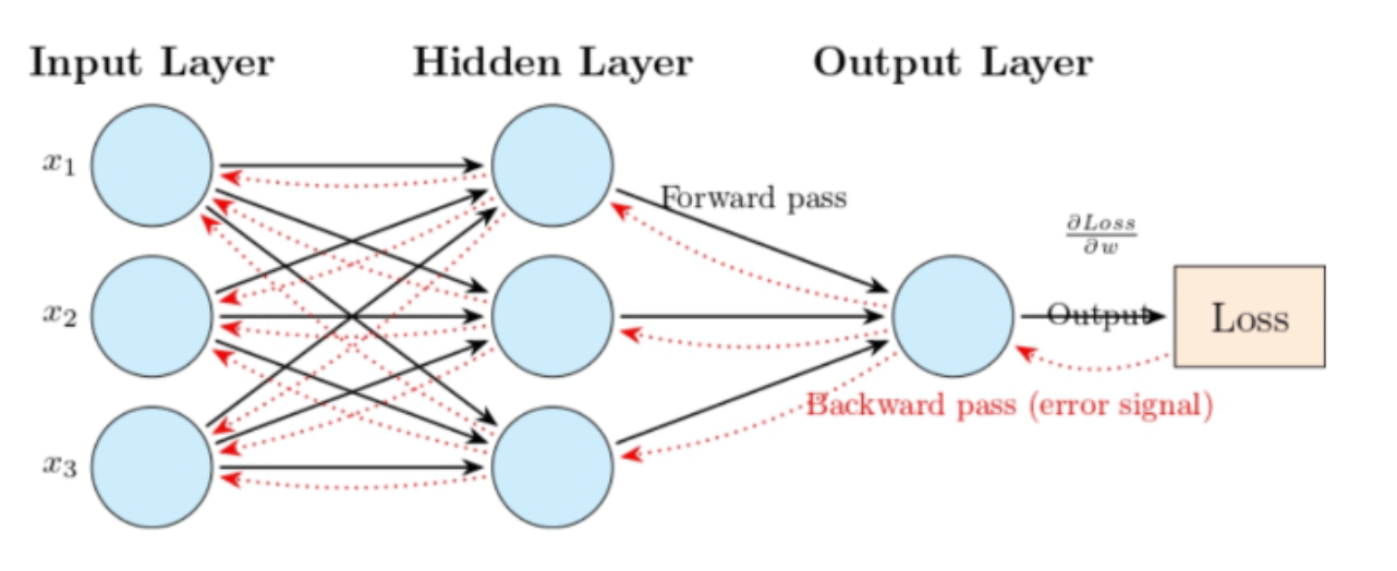
- Activations: Intermediate outputs produced by each layer during the forward pass. Stored during training so gradients can be computed.
- Gradients: Values calculated during backpropagation that tell the model how to update its weights.
- Optimizer States: Additional tensors (like momentum, variance) that optimizers such as Adam or SGD maintain to stabilize training.
- Weights (Parameters): The learnable values inside a model. Updated during training to reduce loss.
- KV Cache (Key-Value Cache): In transformers, a memory structure used during inference to store past attention states for faster decoding.
Additional Useful Concepts
- Compute-Bound vs Memory-Bound Workloads: Compute-bound = limited by math operations, Memory-bound = limited by data movement
Different tasks bottleneck differently. - Epoch: One full pass through the entire training dataset.
- Batch Size: Number of samples processed in a single forward/backward pass.
- Model Size: The number of parameters in the model. Larger models are more powerful but more expensive to train.
Below is a detailed Python code example to demonstrate these core concepts, like FLOPs, tensors, matrix multiplications, throughput, GPU hours, mixed precision, and quantization, all in a practical, runnable form.
PyTorch Lightning Version
import torch
import torch.nn as nn
from torch.utils.data import DataLoader, TensorDataset
import pytorch_lightning as pl
from pytorch_lightning.callbacks import LearningRateMonitor
from pytorch_lightning.strategies import DDPStrategy
from torch.cuda.amp import GradScaler
import time

# -------------------------------------------
# Mixed Precision + Basic Lightning Model
# -------------------------------------------

class LightningMLP(pl.LightningModule):
    def __init__(self):
        super().__init__()
        self.model = nn.Sequential(
            nn.Linear(1024, 2048),
            nn.ReLU(),
            nn.Linear(2048, 1024)
        )
        self.loss_fn = nn.MSELoss()

    def forward(self, x):
        return self.model(x)

    def training_step(self, batch, batch_idx):
        x, y = batch
        with torch.cuda.amp.autocast():     # Mixed precision forward pass
            preds = self.model(x)
            loss = self.loss_fn(preds, y)
        self.log("train_loss", loss)
        return loss

    def configure_optimizers(self):
        return torch.optim.Adam(self.parameters(), lr=1e-3)

# -------------------------------------------
# Dataset
# -------------------------------------------

X = torch.randn(10_000, 1024)
Y = torch.randn(10_000, 1024)
dataset = TensorDataset(X, Y)
loader = DataLoader(dataset, batch_size=32, shuffle=True)

# -------------------------------------------
# Throughput Measurement
# -------------------------------------------

dummy_batch = next(iter(loader))[0]

start = time.time()
for _ in range(200):
    _ = dummy_batch @ dummy_batch.T
end = time.time()

throughput = (200 * dummy_batch.shape[0]) / (end - start)
print(f"Matrix Throughput: {throughput:.2f} samples/sec")

# -------------------------------------------
# Trainer with Mixed Precision
# -------------------------------------------

trainer = pl.Trainer(
    max_epochs=2,
    accelerator="gpu",
    devices=1,
    precision=16,              # Mixed Precision
    callbacks=[LearningRateMonitor(logging_interval="epoch")],
)

model = LightningMLP()
trainer.fit(model, loader)

# -------------------------------------------
# GPU Hours Example
# -------------------------------------------

num_gpus = 4
training_time_hours = 6

gpu_hours = num_gpus * training_time_hours
print(f"Total GPU Hours: {gpu_hours} GPU-hours")

# -------------------------------------------
# INT8 Quantization (Post-Training)
# -------------------------------------------

model_cpu = model.to("cpu")
quantized = torch.ao.quantization.quantize_dynamic(
    model_cpu, {nn.Linear}, dtype=torch.qint8
)

test_input = torch.randn(1, 1024)
out = quantized(test_input)
print("Quantized Output Shape:", out.shape)

# -------------------------------------------
# KV Cache Example
# -------------------------------------------

num_heads = 8
seq_len = 16
head_dim = 64

kv_cache = {
    "key": torch.randn(num_heads, seq_len, head_dim),
    "value": torch.randn(num_heads, seq_len, head_dim),
}

print("KV Cache Shapes:", {k: v.shape for k, v in kv_cache.items()})
The PyTorch Lightning code shows how to train a small neural network using mixed precision (FP16). Lightning handles most of the training, so you only write the model and choose the precision.
This code demonstrates:
- How mixed precision speeds up training
- How Lightning simplifies training loops
- How GPUs automatically use Tensor Cores for faster matrix multiplications
TensorFlow/Keras Version
import tensorflow as tf
from tensorflow import keras
import time

# Enable mixed precision globally
mixed_precision = tf.keras.mixed_precision.set_global_policy("mixed_float16")

# ------------------------------------------------------
# Simple MLP with Mixed Precision
# ------------------------------------------------------

inputs = keras.Input(shape=(1024,))
x = keras.layers.Dense(2048, activation="relu")(inputs)
outputs = keras.layers.Dense(1024)(x)

model = keras.Model(inputs, outputs)

model.compile(
    optimizer=keras.optimizers.Adam(),
    loss="mse"
)

# ------------------------------------------------------
# Dataset
# ------------------------------------------------------

X = tf.random.normal((10000, 1024))
Y = tf.random.normal((10000, 1024))

dataset = tf.data.Dataset.from_tensor_slices((X, Y)).batch(32)

# ------------------------------------------------------
# FLOPs Calculation Example
# ------------------------------------------------------

def compute_flops(M, N, K):
    return 2 * M * N * K

flops = compute_flops(2048, 2048, 2048)
print(f"FLOPs for matmul: {flops/1e9:.2f} GFLOPs")

# ------------------------------------------------------
# Measure Throughput
# ------------------------------------------------------

batch = next(iter(dataset))

start = time.time()
for _ in range(200):
    _ = tf.matmul(batch[0], batch[0], transpose_b=True)
end = time.time()

throughput = (200 * batch[0].shape[0]) / (end - start)
print(f"TF Throughput: {throughput:.2f} samples/sec")

# ------------------------------------------------------
# Train
# ------------------------------------------------------

model.fit(dataset, epochs=2)

# ------------------------------------------------------
# GPU Hours Example
# ------------------------------------------------------

num_gpus = len(tf.config.list_physical_devices("GPU"))
training_time_hours = 4
gpu_hours = num_gpus * training_time_hours

print("GPU Hours:", gpu_hours)

# ------------------------------------------------------
# Post-Training Quantization (INT8)
# ------------------------------------------------------

converter = tf.lite.TFLiteConverter.from_keras_model(model)
converter.optimizations = [tf.lite.Optimize.DEFAULT]  # Enables INT8
tflite_model = converter.convert()

print("TFLite INT8 model size:", len(tflite_model) / 1024, "KB")

# ------------------------------------------------------
# KV Cache Example
# ------------------------------------------------------

num_heads = 8
seq_len = 16
head_dim = 64

kv_cache = {
    "k": tf.random.normal((num_heads, seq_len, head_dim)),
    "v": tf.random.normal((num_heads, seq_len, head_dim)),
}

print("KV Cache Shapes:", {k: v.shape for k, v in kv_cache.items()})
The TensorFlow/Keras code demonstrates the same concept, training a model with mixed precision to accelerate and improve the efficiency of training. TensorFlow enables mixed precision at the global level and automatically uses FP16 where safe.
This code demonstrates:
- How to use mixed precision in TensorFlow
- How models train faster with less GPU memory
- How TF automatically handles loss scaling and FP32 stability
Understanding the Carbon Footprint of Deep Learning
Deep learning models are powerful, but they also consume a lot of energy. This energy use is the main reason why their carbon footprint is rising. Since a large part of global electricity still comes from fossil fuels, every extra watt of power used by GPUs eventually converts into more CO₂ being emitted somewhere in the world.
Training large models is one of the biggest contributors to this energy consumption. Models like Transformers and Vision Transformers (ViTs) perform huge numbers of matrix multiplications for every token or image patch. They also process the full dataset multiple times, often using many GPUs running in parallel for days or even weeks. All these GPUs working continuously consume a lot of electricity.
Several technical factors make deep learning even more energy-intensive. Model size is a major contributor: larger models need more computation. Sequence length, especially in Transformers, can cause computation to grow quadratically; doubling the sequence length can require four times the compute. Batch size also affects power usage; larger batches can speed up training but require more power per step. On top of that, hardware inefficiencies such as older GPUs, poor cooling, or slow memory access can further increase energy consumption.
All this power usage directly translates into CO₂ emissions. Since much of the world still relies on coal, natural gas, and other fossil fuels for electricity, high GPU consumption means more fossil fuels are burned to meet the demand.
The chain is simple:
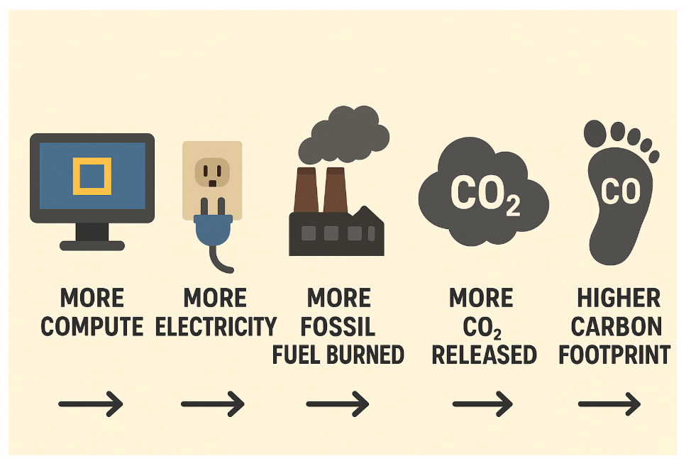
This is why improving energy efficiency in deep learning is becoming a priority for both companies and researchers.
One of the most effective ways to reduce this carbon impact is precision scaling. Precision refers to how many bits are used to represent numbers during computation. For example, FP32 uses 32 bits, while FP16 uses 16 bits, half the size. FP32 requires more memory bandwidth and heavier computation, which leads to more energy use. FP16, on the other hand, is lighter and allows the GPU to process data faster and more efficiently.
You can think of it like lifting weights: FP32 is like lifting a 10 kg dumbbell, while FP16 is like lifting a 5 kg one.

The movement is the same, but FP16 requires less effort every time. Over millions or billions of operations, this reduces power consumption significantly.
Modern GPUs have specialized hardware, Tensor Cores, designed to run FP16 and even lower precisions like INT8 and INT4 extremely efficiently. By switching to lower precision formats wherever possible, we can greatly reduce the energy required for both training and inference, helping cut down carbon emissions without sacrificing model performance.

What Is Precision Scaling?
Precision scaling is a technique that changes the numerical precision (number of bits) used to represent numbers in deep learning models during training, inference or both. In deep learning, every weight, activation, gradient, and any other value is stored as a numerical representation. These numbers can be represented in different precisions, such as:
- FP32 (32-bit float)
- FP16 / BF16 (16-bit float)
- FP8 (8-bit float)
- INT8 (8-bit integer)
- INT4 (4-bit integer)…all the way down to binary (1-bit).
Precision scaling simply means using fewer bits where possible.
- Precision scaling aims to reduce compute costs, as fewer bits mean smaller numbers, which in turn leads to faster matrix multiplications.
- Precision scaling also reduces memory usage, as lower precision leads to smaller tensors, resulting in less GPU memory and lower memory bandwidth requirements.
How Deep Learning Uses Numerical Formats
Neural networks consist of:
- Weights
- Activations
- Gradients
- Optimizer states
- KV cache (for transformers)
as floating-point numbers or integers. Traditionally, this was FP32, but now the trend is:
- Training → BF16 / FP16 / FP8
- Inference → INT8 / INT4 / even INT3
Different parts of a model can use different precisions depending on:
- Stability
- Hardware support
- Bottlenecks (compute vs memory)
How Precision Scaling Improves Energy Efficiency
As we understood, Precision scaling is the practice of reducing numerical bit-width during training or inference, directly improving computational efficiency and lowering energy consumption across modern deep learning workloads. As large models continue to grow in size, lowering precision has become one of the most impactful strategies for reducing both carbon footprint and operational cost.
Reduced Computational Load
Lower-precision formats (such as FP16, BF16, FP8, or INT8) use fewer bits per multiply–accumulate (MAC) operation, which significantly reduces the amount of work performed by GPU compute units.
- Fewer bits → fewer FLOPs needed per operation
- Matrix multiplications execute faster, shortening training cycles.
- Reduced arithmetic complexity also improves GPU occupancy.
As a result, a training step executed in FP8 or BF16 often completes much faster than FP32, improving overall training throughput.
Lower Memory Bandwidth Requirements
Memory access is one of the largest contributors to power draw on modern accelerators. Using lower-precision tensors reduces the number of bytes that must move between GPU memory and compute cores.
For example:
- INT8 tensors use 4× less memory than FP32
- Lower precision leads to fewer memory transactions and reduced latency
- Improves efficiency for bandwidth-bound workloads such as inference and long-sequence decoding
This reduction in data movement directly decreases energy consumption, especially at scale.
Higher Throughput
Modern accelerators like the NVIDIA H100 and NVIDIA A100 provide far higher peak performance when computations are performed in low precision.
- Tensor Cores deliver significantly higher TFLOPs for FP16/FP8/INT8 than FP32
- Higher throughput means each training step or inference run completes using less wall-clock time and less total energy
In inference workloads, this translates to:
- Faster responses
- Lower energy drawn per request
- More queries handled per watt
Real-World Reduction in Carbon Emissions
Because compute time is directly tied to power consumption, reducing precision leads to a meaningful environmental impact.
Shorter training time = fewer GPU-hours = lower total energy usage
Major AI labs have already adopted mixed-precision or low-precision training to cut operational costs and carbon emissions. Companies such as Meta, Google, and OpenAI extensively use lower-precision formats (BF16, FP8, INT8) in their production pipelines, and new hardware is accelerating the push toward even lower bit-widths.
Mixed Precision Training
Mixed precision training was introduced to make deep learning faster and more efficient without sacrificing accuracy. As models and datasets grew larger, training in full FP32 became slow and memory-heavy. Mixed precision solves this by using lower-precision formats like FP16 for most operations, which reduces memory use and increases math throughput, while still keeping critical values like weights and accumulations in FP32 to preserve numerical stability.
With techniques such as loss scaling, mixed precision delivers the same accuracy as FP32 training but with significantly higher speed and lower resource requirements, making it ideal for modern large-scale AI workloads.
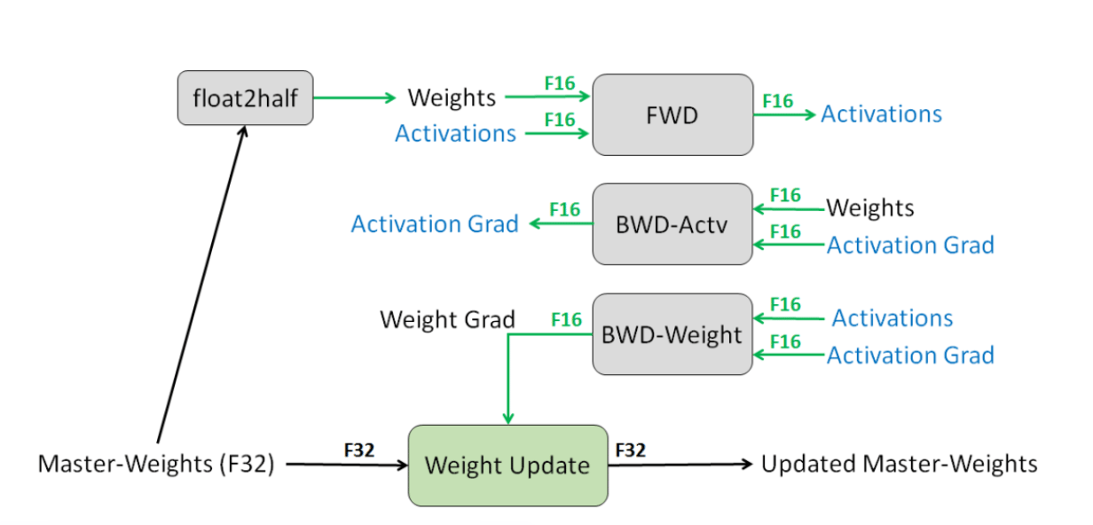
Mixed precision training is a technique where deep learning models use a combination of FP16 (half precision) and FP32 (single precision) to make training faster and more memory-efficient while still keeping the model numerically stable. Most of the heavy computations, like forward and backward passes, run in FP16, which is much faster and uses less memory. But important values such as master weights and accumulations are kept in FP32 to avoid precision loss and ensure training stays accurate. This balance gives you the speed benefits of FP16 without hurting model quality.
Modern frameworks make this easy: PyTorch AMP (Automatic Mixed Precision) and the TensorFlow mixed precision API both provide built-in support, automatically choosing which operations run in FP16 and which stay in FP32, so you get faster training with almost no extra effort.
What is Loss Scaling in mixed-precision training?
Loss scaling is a technique used in mixed-precision training to prevent gradients from becoming too small to represent in FP16. Because FP16 has a limited dynamic range, many gradient values, especially very small negative ones, get rounded down to zero, which harms learning. To fix this, we multiply (scale) the loss by a constant factor before backpropagation. Since backpropagation follows the chain rule, all gradients get scaled up by the same amount. This pushes small gradients into the FP16-representable range so they don’t vanish. After backpropagation, we unscale the gradients before updating the FP32 master weights, ensuring the update size stays correct.
In short:
- Scale the loss → gradients become larger → FP16 can represent them
- Unscale gradients → correct update size → stable training
Choosing the scaling factor can be manual or automatic (dynamic scaling). If the factor is too large, gradients overflow to NaN/Inf, so frameworks detect this and skip the update for that iteration. But when done correctly, loss scaling prevents tiny gradients from disappearing and allows FP16 training to match FP32 accuracy.
Quantization
Quantization is a model-compression technique that reduces the precision of numbers used to store weights and activations in a neural network. Instead of 32-bit floating-point (FP32), the model uses low-bit integer formats like INT8 or INT4, where each number requires far fewer bits.
The idea is straightforward: Neural networks don’t need full 32-bit precision to make accurate predictions. So we “compress” the numbers by mapping them to a smaller integer range + a scaling factor. This drastically reduces model size, memory consumption, and compute cost, without heavily affecting accuracy.
Quantization is now a standard technique for deploying large models efficiently on servers, edge devices, and GPUs.
-
Post-training quantization (PTQ) is the simplest approach, where a fully-trained model is converted to lower precision without retraining. PTQ is fast and easy to apply, requiring only a small calibration dataset to estimate activation ranges. Although PTQ may cause a slight drop in accuracy, it dramatically reduces memory footprint and speeds up inference, making it a popular default choice for deployment.
-
Quantization-aware training (QAT) goes a step further by simulating quantization effects during training. The model “learns” to operate under low-precision constraints, adjusting weights to compensate for rounding errors. Because the model adapts to INT8 or INT4 arithmetic during training, QAT typically achieves much better accuracy than PTQ, especially for sensitive tasks like object detection or generative modeling. QAT is more compute-intensive upfront, but it produces highly optimized quantized models.
One of the biggest advantages of quantization is its ability to drastically reduce energy use. Integer operations (INT8/INT4) require far fewer transistors, memory accesses, and power compared to floating-point math. As a result, quantized models can run many times faster and with significantly lower energy consumption—critical for mobile, IoT, and large-scale inference workloads.
Modern tooling makes quantization much easier. The Hugging Face Optimum library provides optimized INT8 and INT4 pipelines for Transformers, enabling quick conversion with ONNX Runtime or Intel Neural Compressor backends. Meanwhile, Quanto, a lightweight quantization backend for PyTorch, enables fast quantization workflows with native PyTorch compatibility and supports dynamic, static, and integer-only quantization modes. Together, these tools simplify the process of deploying smaller, greener, and faster AI models.
To understand more about quantization techniques, we have linked the detailed blog in our resources section.
Comparing Energy Savings Across Precision
| Precision | Relative Compute Cost | Memory Use | Energy Savings |
|---|---|---|---|
| FP32 | High | High | Baseline |
| FP16/BF16 | ~2× faster | 50% memory | ~30–50% less energy |
| FP8 | ~4× faster | 75% less memory | Up to 60% less energy |
| INT8 | ~4–6× faster | 75% less memory | Up to 70% less energy |
| INT4 | ~8× faster | 87% less memory | Up to 80% less energy |
Practical Guide: Implementing Precision Scaling
Short Checklist for Training
- Allow AMP (automatic mixed precision) for immediate speed & memory gains.
- Use framework-level mixed-precision (FP16/BF16) where supported.
- When available, try FP8 or libraries (NVIDIA Transformer Engine) for extra savings.
- Validate model stability (loss scaling, gradient checks) when lowering precision.
PyTorch — enable AMP (FP16/BF16)
# PyTorch: simple mixed-precision training loop with AMP
import torch
from torch import nn, optim
from torch.cuda.amp import autocast, GradScaler

model = nn.Sequential(nn.Linear(1024, 2048), nn.ReLU(), nn.Linear(2048, 1024)).cuda()
opt = optim.Adam(model.parameters(), lr=1e-3)
scaler = GradScaler()  # for stable FP16 training

for epoch in range(num_epochs):
    for x, y in dataloader:
        x, y = x.cuda(), y.cuda()
        opt.zero_grad()
        with autocast():              # forward in mixed precision
            pred = model(x)
            loss = ((pred - y) ** 2).mean()
        scaler.scale(loss).backward() # scale gradients
        scaler.step(opt)
        scaler.update()
Notes:
- Use
autocast()for FP16; on platforms that support BF16, set dtype accordingly. - For very large models, use gradient accumulation and careful loss-scaling.
PyTorch — FP8 / low-precision (how to start)
- FP8 is hardware-dependent (e.g., H100/Hopper). Use vendor libraries (NVIDIA Transformer Engine / custom kernels) when available.
- Typical steps: install vendor SDK → replace core ops (GEMM/MatMul/LayerNorm) with vendor FP8-accelerated ops → run sanity checks.
- Example (outline):
# pseudocode
from transformer_engine import fp8_layer, cast_to_fp8
x_fp8 = cast_to_fp8(x)
out = fp8_layer(x_fp8, weight_fp8)
TensorFlow / Keras — mixed precision
import tensorflow as tf
from tensorflow import keras

# Enable policy globally (auto chooses BF16 on TPUs / supported GPUs)
tf.keras.mixed_precision.set_global_policy('mixed_float16')

model = keras.Sequential([
    keras.layers.Dense(2048, activation='relu', input_shape=(1024,)),
    keras.layers.Dense(1024)
])
model.compile(optimizer='adam', loss='mse')
model.fit(dataset, epochs=2)
Notes
- Keras handles loss scaling automatically for
mixed_float16. - For BF16 on cloud TPUs or supported GPUs,
mixed_bfloat16is an option.
Short Checklist for Inference
- Try post-training quantization (INT8/INT4) first — fastest path to memory savings.
- If PTQ hurts accuracy, use quantization-aware training (QAT) to adapt weights.
- Export to ONNX, then optimize with TensorRT or ONNX Runtime (ORT) for maximum throughput.
- Measure accuracy vs energy/latency trade-offs before wide deployment.
PyTorch → ONNX → TensorRT (export)
import torch

# assume `model` on CPU / eval mode
model.eval()
dummy = torch.randn(1, 1024)
torch.onnx.export(model.cpu(), dummy, "model.onnx",
                  input_names=["input"], output_names=["output"],
                  opset_version=17, do_constant_folding=True)
ONNX Runtime — quantize ONNX model (dynamic/static)
from onnxruntime.quantization import quantize_dynamic, QuantType

quantize_dynamic("model.onnx", "model_int8.onnx", weight_type=QuantType.QInt8)
Load and run:
import onnxruntime as ort
sess = ort.InferenceSession("model_int8.onnx", providers=['CUDAExecutionProvider'])
out = sess.run(None, {'input': dummy_np})
TensorFlow Lite (mobile/edge INT8)
import tensorflow as tf
converter = tf.lite.TFLiteConverter.from_keras_model(model)
converter.optimizations = [tf.lite.Optimize.DEFAULT]
# (optionally supply representative dataset for full-int8)
tflite_model = converter.convert()
open("model.tflite","wb").write(tflite_model)
FAQ’s
- 1. What is FP32, and why is it used in deep learning?
FP32, or 32-bit floating-point precision, is the standard numerical format used in most deep learning models. Its high numerical stability makes it ideal for training complex networks such as Transformers and CNNs. Because FP32 captures very small decimal variations, it supports stable gradient updates and prevents training divergence. However, its high memory footprint and computational cost make it energy-intensive, which is why lower-precision formats are becoming more popular.
- 2. What does “carbon footprint” mean in the context of AI workloads?
The carbon footprint refers to the total greenhouse gas emissions generated from the electricity used to train and run machine learning models. Large models can consume massive amounts of energy, especially when using high-precision math on GPUs for long training cycles. This energy often comes from non-renewable sources, contributing to global emissions. Reducing precision, optimizing compute, and using more efficient hardware can dramatically lower the carbon footprint of AI systems.
- 3. What is mixed precision training?
Mixed precision training combines two numerical formats, usually FP16 and FP32, to achieve both speed and stability. FP16 is used for most operations to accelerate computation and reduce memory usage, while FP32 is kept for sensitive calculations like loss scaling and gradient accumulation. Frameworks like PyTorch AMP and TensorFlow’s mixed precision API automate this process, ensuring accuracy is preserved. Mixed precision is now one of the most widely adopted methods to improve efficiency without sacrificing model performance.
- 4. What are the different types of precision scaling techniques?
Precision scaling involves adjusting numerical formats to make computation more efficient. The most common forms include mixed precision (FP16 + FP32) for training acceleration, reduced precision inference (such as FP8, INT8, or INT4) for deployment efficiency, and quantization, which compresses models by lowering weight and activation precision. Each technique offers its own trade-offs between speed, accuracy, and energy consumption. Together, they form the core toolkit for energy-efficient deep learning.
- 5. How does reducing precision lower energy consumption?
Lower-precision formats require fewer bits to store numbers, which reduces the amount of memory transferred during computation, a major source of energy usage. Integer operations like INT8 or INT4 also consume far less power than floating-point math because they use simpler circuits and fewer computational steps. This results in faster inference speeds, smaller models, and dramatically reduced energy draw from hardware. At scale, precision reduction can significantly lower the environmental impact of AI workloads.
- 6. What is quantization, and how does it differ from mixed precision?
Quantization converts model weights and activations from floating-point values to low-precision integer values like INT8 or INT4. Unlike mixed precision, which still uses floating-point math, quantization replaces many operations with integers, offering much higher efficiency. It can be applied post-training (PTQ) or during training (QAT) to preserve accuracy. Quantized models use far less memory and power, making quantization ideal for edge devices, large-scale inference, or carbon-conscious deployments.
- 7. Does precision scaling affect model accuracy?
Precision scaling can introduce rounding errors and reduce representational granularity, which may slightly affect accuracy—especially for small models or sensitive tasks. However, modern techniques like loss scaling, quantization-aware training, and FP8 training greatly mitigate these issues. In many cases, models maintain near-identical accuracy while using a fraction of the compute. The small accuracy trade-off is often worth the large gains in speed, cost savings, and reduced environmental impact.
- 8. Can precision scaling be applied to any model architecture?
Most modern architectures, including Transformers, CNNs, RNNs, and diffusion models, support mixed precision and quantization. Frameworks and hardware accelerators now offer built-in support, making adoption straightforward. However, certain older architectures or custom operations may require tuning to avoid numerical instability. With proper tooling, nearly all widely used deep learning models can benefit from precision scaling to improve efficiency.
Conclusion
Precision scaling is quickly becoming one of the effective ways to reduce the model complexities and energy requirements for deep learning tasks. By shifting from full FP32 to lighter formats like FP16, FP8, INT8, or INT4, we can cut training and inference costs while shrinking the carbon footprint of modern AI systems. It’s a simple idea with a huge impact: faster models, lower bills, and a more sustainable path for scaling AI.
Of course, it’s not perfect. Extremely low precision can hurt accuracy, framework support can be inconsistent, and some hardware still struggles with advanced quantization. Certain fields, like scientific computing, also need the stability of higher precision. But despite these challenges, precision scaling remains a powerful strategy for building efficient, responsible, and future-ready AI.
Thanks for learning with the DigitalOcean Community. Check out our offerings for compute, storage, networking, and managed databases.
About the author
With a strong background in data science and over six years of experience, I am passionate about creating in-depth content on technologies. Currently focused on AI, machine learning, and GPU computing, working on topics ranging from deep learning frameworks to optimizing GPU-based workloads.
Still looking for an answer?
This textbox defaults to using Markdown to format your answer.
You can type !ref in this text area to quickly search our full set of tutorials, documentation & marketplace offerings and insert the link!
 This work is licensed under a Creative Commons Attribution-NonCommercial- ShareAlike 4.0 International License.
Become a contributor for community
Get paid to write technical tutorials and select a tech-focused charity to receive a matching donation.

DigitalOcean Documentation
Full documentation for every DigitalOcean product.

Resources for startups and AI-native businesses
The Wave has everything you need to know about building a business, from raising funding to marketing your product.
The developer cloud
Scale up as you grow — whether you're running one virtual machine or ten thousand.

Start building today
From GPU-powered inference and Kubernetes to managed databases and storage, get everything you need to build, scale, and deploy intelligent applications.
